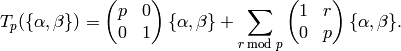
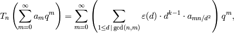
Modular Forms of Weight 2
We saw in Chapter Modular Forms of Level 1 (especially
Section Structure Theorem for Level 1 Modular Forms) that we can compute each space
 explicitly. This involves computing Eisenstein
series
explicitly. This involves computing Eisenstein
series  and
and  to some precision, then forming the basis
 for .
In this chapter we consider the more general problem of computing
for .
In this chapter we consider the more general problem of computing
 , for any positive integer
  . Again we have a
decomposition
. Again we have a
decomposition

where  is spanned by generalized
Eisenstein
series and is the space of cusp forms,
i.e., elements of
is spanned by generalized
Eisenstein
series and is the space of cusp forms,
i.e., elements of  that vanish at all cusps.
In Chapter Eisenstein Series and Bernoulli Numbers we compute the space
in a similar way to how we computed . On the other
hand, elements of often cannot be written as sums
or products of generalized Eisenstein series. In fact, the structure
of is, in general, much more complicated than that
of . For example, when  is a prime,
 has dimension
  , whereas
  has dimension about
  .
.
Fortunately an idea of Birch, which he called modular symbols, provides a
method for computing and indeed for much more
that is relevant to understanding special values of  -functions.
Modular symbols are also a powerful theoretical tool. In this
chapter, we explain how is related to modular
symbols and how to use this relationship to explicitly compute a
basis for . In Chapter General Modular Symbols we will
introduce more general modular symbols and explain how to use them to
compute
-functions.
Modular symbols are also a powerful theoretical tool. In this
chapter, we explain how is related to modular
symbols and how to use this relationship to explicitly compute a
basis for . In Chapter General Modular Symbols we will
introduce more general modular symbols and explain how to use them to
compute  ,
,  and
and  for
any integers
for
any integers  and and character
  .
.
Section Hecke Operators contains a very brief summary of basic facts
about modular forms of weight  , modular curves, Hecke operators,
and integral homology. Section Modular Symbols introduces modular
symbols and describes how to compute with them. In
Section Computing the Boundary Map we talk about how to cut out the
subspace of modular symbols corresponding to cusp forms using the
boundary map. Section Computing a Basis for is about a straightforward
method to compute a basis for using modular
symbols, and Section Computing Using Eigenvectors outlines a more
sophisticated algorithm for computing newforms that uses
Atkin-Lehner theory.
, modular curves, Hecke operators,
and integral homology. Section Modular Symbols introduces modular
symbols and describes how to compute with them. In
Section Computing the Boundary Map we talk about how to cut out the
subspace of modular symbols corresponding to cusp forms using the
boundary map. Section Computing a Basis for is about a straightforward
method to compute a basis for using modular
symbols, and Section Computing Using Eigenvectors outlines a more
sophisticated algorithm for computing newforms that uses
Atkin-Lehner theory.
Before reading this chapter, you should have read Chapter Modular Forms and Chapter Modular Forms of Level 1. We also assume familiarity with algebraic curves, Riemann surfaces, and homology groups of compact Riemann surfaces.
Hecke Operators
Recall from Chapter Modular Forms that the group  acts on
 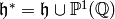 by linear fractional transformations.
The quotient
by linear fractional transformations.
The quotient  is a Riemann surface, which
we denote by
is a Riemann surface, which
we denote by  . See [DS05, Ch. 2] for a
detailed description of the topology on . The Rieman surface
also has a canonical structure of algebraic curve over
. See [DS05, Ch. 2] for a
detailed description of the topology on . The Rieman surface
also has a canonical structure of algebraic curve over  ,
as is explained in [DS05, Ch. 7] (see also
[Shi94, Section 6.7]).
,
as is explained in [DS05, Ch. 7] (see also
[Shi94, Section 6.7]).
Recall from Section Modular Forms of Any Level that a cusp form of weight
for is a function  on
on  such that
  defines
a holomorphic differential on .
Equivalently, a cusp form is a holomorphic function on such
that
defines
a holomorphic differential on .
Equivalently, a cusp form is a holomorphic function on such
that
- the expression is invariant
under replacing
 by
by  for each
  and
and  vanishes at every cusp for .
The space of weight cusp forms on
is a finite-dimensional complex vector space, of dimension equal to
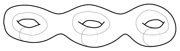
the genus  of . The space
  is a compact
oriented Riemann surface, so it is a -dimensional oriented real
manifold, i.e., is a -holed torus (see
Figure 3.1).
is a compact
oriented Riemann surface, so it is a -dimensional oriented real
manifold, i.e., is a -holed torus (see
Figure 3.1).
Condition (b) in the definition of means that has a Fourier
expansion about each element of  . Thus, at
  we have
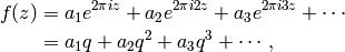
where, for brevity, we write  .
.
Example 3.1
Let  be the elliptic curve defined by the equation
 .
Let
.
Let 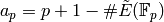 , where
  is the reduction of mod (note that for the
primes that divide the conductor of we have
is the reduction of mod (note that for the
primes that divide the conductor of we have  ,
,  ).2
For
).2
For  composite, define
  using the relations at the
end of Section Computing Using Eigenvectors.
using the relations at the
end of Section Computing Using Eigenvectors.
Then the Shimura-Taniyama conjecture asserts that
is the  -expansion of an element of
  . This
conjecture, which is now a theorem (see
[BCDT01]), asserts that any
-expansion constructed as above from an elliptic curve over
is a modular form. This conjecture was mostly proved first by
Wiles [Wil95] as a key step in the proof of Fermat’s
last theorem.
. This
conjecture, which is now a theorem (see
[BCDT01]), asserts that any
-expansion constructed as above from an elliptic curve over
is a modular form. This conjecture was mostly proved first by
Wiles [Wil95] as a key step in the proof of Fermat’s
last theorem.
Just as is the case for level modular forms (see
Section Hecke Operators) there are commuting Hecke operators  that act on . To define them
conceptually, we introduce an interpretation of the modular curve
as an object whose points parameterize elliptic curves
with extra structure.
that act on . To define them
conceptually, we introduce an interpretation of the modular curve
as an object whose points parameterize elliptic curves
with extra structure.
Proposition 3.2
The complex points of
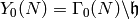 are in natural bijection with
isomorphism classes of pairs
are in natural bijection with
isomorphism classes of pairs  , where is an elliptic
curve over
, where is an elliptic
curve over  and
and  is a cyclic subgroup of
  of
order . The class of the point
of
order . The class of the point  corresponds to
the pair
corresponds to
the pair
Proof
See Exercise 3.1.
Suppose and are coprime positive integers. There are two
natural maps  and
and  from
from  to
to  ; the
first, , sends
; the
first, , sends  to
to  , where
 is the unique cyclic subgroup of of order , and the
second, , sends to
is the unique cyclic subgroup of of order , and the
second, , sends to  , where
  is the
unique cyclic subgroup of of order . These maps extend in a
unique way to algebraic maps from
is the
unique cyclic subgroup of of order . These maps extend in a
unique way to algebraic maps from  to :
to :
(1)![\xymatrix{ & X_0(n\cdot N) \ar[dl]_{\pi_2}\ar[dr]^{\pi_1}\\
X_0(N) & & X_0(N).}](_images/math/93b0b68694aa8ee4b37d3a3dec9f4ac500068856.png)
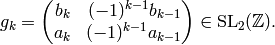
The  Hecke operator
  is
is  ,
where
,
where  and
and  denote pullback and pushforward
of differentials, respectively. (There is a similar definition
of when
denote pullback and pushforward
of differentials, respectively. (There is a similar definition
of when  .)
Using our interpretation of as differentials
on , this gives an action of Hecke operators on .
One can show that these induce the maps of Proposition 2.31
on -expansions.
.)
Using our interpretation of as differentials
on , this gives an action of Hecke operators on .
One can show that these induce the maps of Proposition 2.31
on -expansions.
Example 3.3
There is a basis of  so that
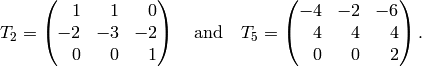
Notice that these matrices commute. Also, the characteristic
polynomial of  is
is  .
.
Homology
The first homology group  is the group of closed
-cycles modulo boundaries of -cycles (formal sums of images of
-simplexes). Topologically is a -holed torus,
where is the genus of . Thus is a free
abelian group of rank
is the group of closed
-cycles modulo boundaries of -cycles (formal sums of images of
-simplexes). Topologically is a -holed torus,
where is the genus of . Thus is a free
abelian group of rank  (see, e.g.,
[Gre81, Ex. 19.30] and [DS05, Section 6.1]),
with two generators corresponding to each hole, as illustrated in the
case
(see, e.g.,
[Gre81, Ex. 19.30] and [DS05, Section 6.1]),
with two generators corresponding to each hole, as illustrated in the
case  in Figure 3.1.
Figure 3.1
The homology of 

The homology of is closely related to modular forms, since
the Hecke operators also act on . The action
is by pullback of homology classes by followed by taking the
image under , where and are as in
(1).
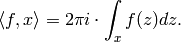
Integration defines a pairing
(2)
Explicitly, for a path  ,
,
Theorem 3.4
The pairing (2) is nondegenerate and Hecke
equivariant in the sense that for every Hecke operator , we
have  .
Moreover, it induces a perfect pairing
.
Moreover, it induces a perfect pairing

This is a special case of the results in Section Pairing Modular Symbols and Modular Forms.
As we will see, modular symbols allow us to make explicit the action
of the Hecke operators on ; the above pairing then
translates this into a wealth of information about cusp forms.
We will also consider the relative homology group
 of
relative to the cusps; it is the same as usual homology, but i
n addition we allow paths with endpoints in the cusps instead of
restricting to closed loops. Modular symbols provide a
“combinatorial” presentation of in terms of paths
between elements of .
of
relative to the cusps; it is the same as usual homology, but i
n addition we allow paths with endpoints in the cusps instead of
restricting to closed loops. Modular symbols provide a
“combinatorial” presentation of in terms of paths
between elements of .
Modular Symbols
Let  be the free abelian group with basis the set of symbols
 with
with  modulo the 3-term
relations
modulo the 3-term
relations

above and modulo any torsion. Since is torsion-free, we have

Warning
The symbols satisfy the relations
 , so order matters. The
notation looks like the set containing two
elements, which strongly (and incorrectly) suggests that the order
does not matter. This is the standard notation in the literature.
, so order matters. The
notation looks like the set containing two
elements, which strongly (and incorrectly) suggests that the order
does not matter. This is the standard notation in the literature.
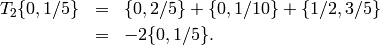
Figure 3.2
The modular symbols and 
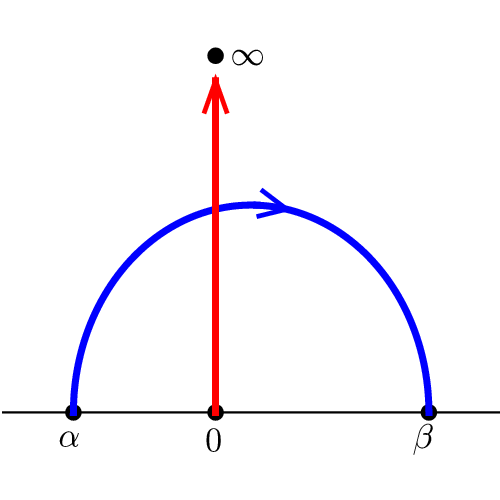
As illustrated in Figure 3.2, we “think of” this
modular symbol as the homology class, relative to the cusps, of a path
from  to
to  in
in  .
.
Define a left action of  on by letting
 act by
and acts on and via the corresponding linear
fractional transformation. The space  of
modular symbols for `\Gamma_0(N)` is the quotient of
by the submodule generated by the infinitely many elements of the form
of
modular symbols for `\Gamma_0(N)` is the quotient of
by the submodule generated by the infinitely many elements of the form
 , for in and in , and modulo
any torsion. A modular symbol for is an element of this
space. We frequently denote the equivalence class of a modular symbol
by giving a representative element.
, for in and in , and modulo
any torsion. A modular symbol for is an element of this
space. We frequently denote the equivalence class of a modular symbol
by giving a representative element.
Example 3.6
Some modular symbols are  no matter what the level is! For
example, since
no matter what the level is! For
example, since  , we have

so

See Exercise 3.2 for a generalization of this observation.
There is a natural homomorphism
(3)
that sends a formal linear combination of geodesic paths in the upper
half plane to their image as paths on . In
[Man72] Manin proved that (3) is an
isomorphism (this is a fairly involved topological argument).
Manin identified the subspace of that is
sent isomorphically onto . Let  denote the free abelian group whose basis is the finite set
 of cusps for
. The boundary map
of cusps for
. The boundary map

sends to  , where
  denotes the basis element of corresponding to
 . The kernel
  of
of  is
the subspace of cuspidal modular symbols. Thus an element of
can be thought of as a linear combination of
paths in whose endpoints are cusps and whose images in
are homologous to a
is
the subspace of cuspidal modular symbols. Thus an element of
can be thought of as a linear combination of
paths in whose endpoints are cusps and whose images in
are homologous to a  -linear combination of closed paths.
Theorem 3.7
The map  above induces a canonical isomorphism

Proof
This is [Man72, Thm. 1.9].
For any (commutative) ring  let
let

and

Proposition 3.8
We have

Proof
We have

Example 3.9
We illustrate modular symbols in the case when  .
Using Sage (below),
which implements the algorithm that we describe below
over , we find that
.
Using Sage (below),
which implements the algorithm that we describe below
over , we find that  has basis
 ,
,  ,
,  .
A basis for the integral homology
.
A basis for the integral homology  is the
subgroup generated by and .
is the
subgroup generated by and .
sage: set_modsym_print_mode ('modular')
sage: M = ModularSymbols(11, 2)
sage: M.basis()
({Infinity,0}, {-1/8,0}, {-1/9,0})
sage: S = M.cuspidal_submodule()
sage: S.integral_basis()     # basis over ZZ.
({-1/8,0}, {-1/9,0})
sage: set_modsym_print_mode ('manin')    # set it back
Computing with Modular Symbols
In this section, we describe a trick of Manin that we will use to prove that spaces of modular symbols are computable.
By Exercise 1.6 the group has finite index in
 . Fix right coset representatives
  for in , so that

where the union is disjoint. For example, when is prime, a list
of coset representatives is

Let
(4)
where  if there is
  such
that
such
that  .
.
Proposition 3.10
There is a bijection between  and the right cosets of
in , which sends a coset representative
and the right cosets of
in , which sends a coset representative
 to the class of
  in .
in .
Proof
See Exercise 3.3.
See Proposition 1.27 for the analogous statement for
 .
.
We now describe an observation of Manin (see
[Man72, Section 1.5]) that is crucial to making
computable. It allows us to write any modular
symbol  as a -linear combination of symbols of
the form
as a -linear combination of symbols of
the form  , where the
  are coset
representatives as above. In particular, the finitely many symbols
are coset
representatives as above. In particular, the finitely many symbols
 generate
.
generate
.
Proposition 3.11
[Manin]
Let be a positive integer and  a set of right coset representatives for in
.
Every
a set of right coset representatives for in
.
Every  is a -linear combination of
.
is a -linear combination of
.
We give two proofs of the proposition. The first is useful for computation (see [Cre97a, Section 2.1.6]); the second (see [MTT86, Section 2]) is easier to understand conceptually since it does not require any knowledge of continued fractions.
Proof
Since

it suffices to consider modular symbols of the form  ,
where the rational number
,
where the rational number  is in lowest terms. Expand
as a continued fraction and consider the successive convergents in
lowest terms:
is in lowest terms. Expand
as a continued fraction and consider the successive convergents in
lowest terms:

where the first two are included formally. Then
so that
Hence
for some  , is of the required special form. Since

this completes the proof.
Proof
As in the first proof it suffices to prove the proposition for any
symbol , where is in lowest terms. We will induct
on  . If
. If  , then the symbol is ,
which corresponds to the identity coset, so assume that
, then the symbol is ,
which corresponds to the identity coset, so assume that  .
Find
.
Find  such that
then  so the matrix

is an element of . Thus  for
some right coset representative
for
some right coset representative  and
and  .
Then
.
Then

as elements of  . By induction,
  is a linear combination of symbols of the form
  ,
which completes the proof.
,
which completes the proof.
Example 3.12
Let , and consider the modular symbol  . We have
so the partial convergents are

Thus, noting as in Example 3.6 that  , we have
![\begin{eqnarray*}
\{0,4/7\} &=& \{0,\infty\} +\{\infty,0\} + \{0,1\}+ \{1,1/2\} + \{1/2,4/7\}\\
&=& \mtwo{1}{-1}{2}{-1}\{0,\infty\} + \mtwo{4}{1}{7}{2}\{0,\infty\}\\
&=& \mtwo{1}{0}{9}{1}\{0,\infty\} + \mtwo{1}{0}{9}{1}\{0,\infty\}\\
&=& 2 \cdot \left[\mtwo{1}{0}{9}{1}\{0,\infty\}\right].
\end{eqnarray*}](_images/math/df96b4bedffaa381a0cf8fea7e2730d49221792f.png)
We compute the convergents of  in Sage as follows (note that
and are excluded):
in Sage as follows (note that
and are excluded):
sage: convergents(4/7)
[0, 1, 1/2, 4/7]
Manin Symbols
As above, fix coset representatives  for
in . Consider formal symbols
for
in . Consider formal symbols ![[r_i]'](_images/math/f3248949fbd8d814e87d3d0ee027b42e504ca808.png) for
for  .
Let
.
Let ![[r_i]](_images/math/fe4443b5e0c478b5971e9b38e034df52a2f22276.png) be the modular symbol
be the modular symbol
 .
We equip the symbols
.
We equip the symbols ![[r_0]',\ldots,[r_m]'](_images/math/5a510fd2153554e9897e39bab594c9a5447f3a8e.png) with a
right action of , which is given by
with a
right action of , which is given by
![[r_i]'.g = [r_j]'](_images/math/b9e5c5c32284dd34d95e519e4ed74f9af75c78fd.png) , where
, where  .
We extend the notation by writing
.
We extend the notation by writing
![[\gamma]' = [\Gamma_0(N)\gamma]' = [r_i]'](_images/math/6344e12d876553fc2b8949edd7855edb688694a7.png) , where
, where
 . Then the right action of
is simply
. Then the right action of
is simply ![[\gamma]'.g = [\gamma g]'](_images/math/91e87d8b819a512de5abcdc06e927e7cdefac8dc.png) .
.
Theorem 1.2 implies that
is generated by the two matrices
 and
and
 .
Note that
.
Note that  from Theorem 1.2 and
 , so
, so 
The following theorem provides us with a finite presentation for the
space of modular symbols.
Theorem 3.13
Consider the quotient  of the free abelian group
on Manin symbols by the subgroup
generated by the elements (for all ):
of the free abelian group
on Manin symbols by the subgroup
generated by the elements (for all ):
![{[r_i]'} + [r_i]'\sigma \qquad\text{ and }\qquad
{[r_i]'} + [r_i]'\tau + [r_i]'\tau^2 ,](_images/math/314bcd4d1b1a3da3c8673fd0949c6cf0aaacbde2.png)
and modulo any torsion. Then there is an isomorphism
given by ![[r_i]' \mapsto [r_i] = r_i \{0,\infty\}](_images/math/48095e5042e5406e0abc8d3999248bad3b9f93bb.png) .
.
Proof
We will only prove that
is surjective; the proof that
Proposition 3.11 implies that
![{[r_i]} + [r_i]\sigma
&= \{r_i(0),r_i(\infty)\} + \{r_i\sigma(0), r_i\sigma(\infty)\}\\
&= \{r_i(0),r_i(\infty)\} + \{r_i(\infty), r_i(0)\} \\
& = 0.](_images/math/4e1a9e5b6492798d9aa7533f3aff8946aec06721.png)
For the second relation we have
![{[r_i]} + [r_i]\tau + [r_i]\tau^2 &=
\{r_i(0),r_i(\infty)\} + \{r_i\tau(0), r_i\tau(\infty)\}
+ \{r_i\tau^2(0), r_i\tau^2(\infty)\} \\
&= \{r_i(0),r_i(\infty)\} + \{r_i(\infty), r_i(1)\}
+ \{r_i(1), r_i(0)\} \\
&= 0.](_images/math/edbcf86ebcfd0afea244a72363786025454a9c94.png)
Example 3.14
By default Sage computes modular symbols spaces over , i.e.,
 .
Sage represents (weight ) Manin symbols as pairs
.
Sage represents (weight ) Manin symbols as pairs  .
Here
.
Here  are integers that satisfy
  ; they define a point
 , hence a right coset of
in (see Proposition 3.10).
, hence a right coset of
in (see Proposition 3.10).
Create  in Sage by typing
ModularSymbols(N, 2).
We then use the Sage command manin_generators to enumerate a list
of generators
in Sage by typing
ModularSymbols(N, 2).
We then use the Sage command manin_generators to enumerate a list
of generators ![[r_0], \ldots, [r_n]](_images/math/3c45597884fce84747ca09bba717f6137f2368f3.png) as in
Theorem 3.13 for several spaces of modular symbols.
as in
Theorem 3.13 for several spaces of modular symbols.
sage: M = ModularSymbols(2,2)
sage: M
Modular Symbols space of dimension 1 for Gamma_0(2)
of weight 2 with sign 0 over Rational Field
sage: M.manin_generators()
[(0,1), (1,0), (1,1)]

sage: M = ModularSymbols(3,2)
sage: M.manin_generators()
[(0,1), (1,0), (1,1), (1,2)]

sage: M = ModularSymbols(6,2)
sage: M.manin_generators()
[(0,1), (1,0), (1,1), (1,2), (1,3), (1,4), (1,5), (2,1),
(2,3), (2,5), (3,1), (3,2)]
Given x=(c,d), the command x.lift_to_sl2z(N)
computes an element of whose lower two entries are
congruent to modulo .
sage: M = ModularSymbols(2,2)
sage: [x.lift_to_sl2z(2) for x in M.manin_generators()]
[[1, 0, 0, 1], [0, -1, 1, 0], [0, -1, 1, 1]]
sage: M = ModularSymbols(6,2)
sage: x = M.manin_generators()[9]
sage: x
(2,5)
sage: x.lift_to_sl2z(6)
[1, 2, 2, 5]
The manin_basis command returns a list of indices into the
Manin generator list such that the corresponding symbols form a basis
for the quotient of the -vector space spanned by Manin symbols
modulo the -term and  -term relations of
Theorem 3.13.
-term relations of
Theorem 3.13.
sage: M = ModularSymbols(2,2)
sage: M.manin_basis()
[1]
sage: [M.manin_generators()[i] for i in M.manin_basis()]
[(1,0)]
sage: M = ModularSymbols(6,2)
sage: M.manin_basis()
[1, 10, 11]
sage: [M.manin_generators()[i] for i in M.manin_basis()]
[(1,0), (3,1), (3,2)]
Thus, e.g., every element of  is a -linear
combination of the three symbols
is a -linear
combination of the three symbols ![[(1,0)]](_images/math/005384eaf1021152f7921bf2a923d964820a6c4f.png) ,
, ![[(3,1)]](_images/math/1df5ca8552c5b09e03a0362de6a171f8db359db8.png) , and
, and ![[(3,2)]](_images/math/0aebb25edfc0cf432472353596c2a84cb3266ff1.png) .
We can write each of these as a modular symbol using the
modular_symbol_rep function.
.
We can write each of these as a modular symbol using the
modular_symbol_rep function.
sage: M.basis()
((1,0), (3,1), (3,2))
sage: [x.modular_symbol_rep() for x in M.basis()]
[{Infinity,0}, {0,1/3}, {-1/2,-1/3}]
The manin_gens_to_basis function returns a matrix whose rows express each Manin symbol generator in terms of the subset of Manin symbols that forms a basis (as returned by manin_basis).
sage: M = ModularSymbols(2,2)
sage: M.manin_gens_to_basis()
[-1]
[ 1]
[ 0]
Since the basis is  , this
means that in
, this
means that in  , we have
![[(0,1)] = -[(1,0)]](_images/math/6582a8bd0f0f9a02824c5b4306bb8d472b4adb65.png) and
and ![[(1,1)] = 0](_images/math/95dd5c55ac10e04864384dc8a5e4e618e7c66ccd.png) .
(Since no denominators are involved, we have in
fact computed a presentation of
.
(Since no denominators are involved, we have in
fact computed a presentation of  .)
.)
To convert a Manin symbol  to an element of a modular
symbols space , use M(x):
to an element of a modular
symbols space , use M(x):
sage: M = ModularSymbols(2,2)
sage: x = (1,0); M(x)
(1,0)
Next consider  :
:
sage: M = ModularSymbols(6,2)
sage: M.manin_gens_to_basis()
[-1  0  0]
[ 1  0  0]
[ 0  0  0]
[ 0 -1  1]
[ 0 -1  0]
[ 0 -1  1]
[ 0  0  0]
[ 0  1 -1]
[ 0  0 -1]
[ 0  1 -1]
[ 0  1  0]
[ 0  0  1]
Recall that our choice of basis for
is ![[(1,0)], [(3,1)], [(3,2)]](_images/math/8efdf6ef121de6e6fc109b3e2d44f8b69d57e292.png) .
Thus, e.g., the first row of this matrix says that
, and the fourth row asserts
that
.
Thus, e.g., the first row of this matrix says that
, and the fourth row asserts
that
![[(1,2)] = -[(3,1)] + [(3,2)]](_images/math/8e42a6f9fd473ddf5d7b6bb2fa5f1922eee4f720.png) .
.
sage: M = ModularSymbols(6,2)
sage: M((0,1))
-(1,0)
sage: M((1,2))
-(3,1) + (3,2)
Hecke Operators
Hecke Operators on Modular Symbols
When is a prime not dividing , define
The Hecke operators are compatible with
the integration pairing  of Section Hecke Operators, in the
sense that
of Section Hecke Operators, in the
sense that 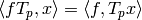 .
When
.
When  , the definition is the same, except that the matrix
 is not included in the sum (see Theorem 1.44).
There is a similar definition of for composite
(see Section General Definition of Hecke Operators).
is not included in the sum (see Theorem 1.44).
There is a similar definition of for composite
(see Section General Definition of Hecke Operators).
 under
under 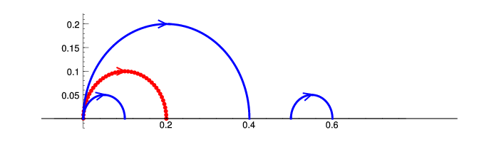
Hecke Operators on Manin Symbols
In [Mer94], L. Merel gives a description of the action of
 directly on Manin symbols (see
Section Hecke Operators on Manin Symbols for details). For example, when
directly on Manin symbols (see
Section Hecke Operators on Manin Symbols for details). For example, when
 and is odd, we have
(5)![T_2([r_i]) = [r_i]\mtwo{1}{0}{0}{2} + [r_i]\mtwo{2}{0}{0}{1}
+ [r_i]\mtwo{2}{1}{0}{1} + [r_i]\mtwo{1}{0}{1}{2}.](_images/math/c3beb09711fdba7ff18c3132ac76eaccb85be341.png)
For any prime, let  be the set of matrices
constructed using the following algorithm (see [Cre97a, Section 2.4]):
be the set of matrices
constructed using the following algorithm (see [Cre97a, Section 2.4]):
Algorithm 3.16
Given a prime , this algorithm outputs a list of  matrices of determinant that can be used to compute the Hecke
operator .
matrices of determinant that can be used to compute the Hecke
operator .
- Output
 .
. - For
 :
:- Let
 ,
,  ,
,  ,
,  ,
,  ,
,  .
. - Output
 .
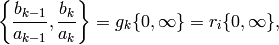
. - As long as
 , do the following:
- Let be the integer closest to
 (if is a half
integer, round away from ).
(if is a half
integer, round away from ). - Let
 ,
,  ,
,  .
. - Set
 , and\
 .
. - Output .
- Let
- Let
Proposition 3.17
Let be as above. Then
for  and
and ![[x]\in \M_2(\Gamma_0(N))](_images/math/dc5f4d802ae7e3f9db73ae5789bf8e4a90a6ea6a.png) a Manin
symbol, we have
a Manin
symbol, we have
![T_p([x]) = \sum_{g \in C_p} [xg].](_images/math/4e86f4de5c3602361f5f70a6dc2a0bfae5df56d6.png)
Proof
See Proposition~2.4.1 of [Cre97a].
There are other lists of matrices, due to Merel, that work even when
(see Section Hecke Operators on Manin Symbols).
The command HeilbronnCremonaList(p), for prime,
outputs the list of matrices from Algorithm 3.16.
  sage: HeilbronnCremonaList(2)
  [[1, 0, 0, 2], [2, 0, 0, 1], [2, 1, 0, 1], [1, 0, 1, 2]]
  sage: HeilbronnCremonaList(3)
  [[1, 0, 0, 3], [3, 1, 0, 1], [1, 0, 1, 3], [3, 0, 0, 1],
  [3, -1, 0, 1], [-1, 0, 1, -3]]
  sage: HeilbronnCremonaList(5)
  [[1, 0, 0, 5], [5, 2, 0, 1], [2, 1, 1, 3], [1, 0, 3, 5],
  [5, 1, 0, 1], [1, 0, 1, 5], [5, 0, 0, 1], [5, -1, 0, 1],
  [-1, 0, 1, -5], [5, -2, 0, 1], [-2, 1, 1, -3],
  [1, 0, -3, 5]]
  sage: len(HeilbronnCremonaList(37))
  128
  sage: len(HeilbronnCremonaList(389))
  1892
  sage: len(HeilbronnCremonaList(2003))
  11662

.. index::
   pair: Sage; Hecke operator `T_2`
Example 3.18
We compute the matrix of
:
sage: M = ModularSymbols(2,2)
sage: M.T(2).matrix()
[1]
Example 3.19
We compute some Hecke operators on :
sage: M = ModularSymbols(6, 2)
sage: M.T(2).matrix()
[ 2  1 -1]
[-1  0  1]
[-1 -1  2]
sage: M.T(3).matrix()
[3 2 0]
[0 1 0]
[2 2 1]
sage: M.T(3).fcp()  # factored characteristic polynomial
(x - 3) * (x - 1)^2
For  we have
  , since
  is
spanned by generalized Eisenstein series (see Chapter Eisenstein Series and Bernoulli Numbers).
is
spanned by generalized Eisenstein series (see Chapter Eisenstein Series and Bernoulli Numbers).
Example 3.20
We compute the Hecke operators on  :
:
sage: M = ModularSymbols(39, 2)
sage: T2 = M.T(2)
sage: T2.matrix()
[ 3  0 -1  0  0  1  1 -1  0]
[ 0  0  2  0 -1  1  0  1 -1]
[ 0  1  0 -1  1  1  0  1 -1]
[ 0  0  1  0  0  1  0  1 -1]
[ 0 -1  2  0  0  1  0  1 -1]
[ 0  0  1  1  0  1  1 -1  0]
[ 0  0  0 -1  0  1  1  2  0]
[ 0  0  0  1  0  0  2  0  1]
[ 0  0 -1  0  0  0  1  0  2]
sage: T2.fcp()     # factored characteristic polynomial
(x - 3)^3 * (x - 1)^2 * (x^2 + 2*x - 1)^2
The Hecke operators commute, so their eigenspace structures are related.
sage: T2 = M.T(2).matrix()
sage: T5 = M.T(5).matrix()
sage: T2*T5 - T5*T2 == 0
True
sage: T5.charpoly().factor()
(x^2 - 8)^2 * (x - 6)^3 * (x - 2)^2
The decomposition of is a list of the kernels of
 , where runs through the irreducible factors of the
characteristic polynomial of and
, where runs through the irreducible factors of the
characteristic polynomial of and  exactly divides this
characteristic polynomial. Using Sage, we find them:
exactly divides this
characteristic polynomial. Using Sage, we find them:
sage: M = ModularSymbols(39, 2)
sage: M.T(2).decomposition()
[
Modular Symbols subspace of dimension 3 of Modular
Symbols space of dimension 9 for Gamma_0(39) of weight
2 with sign 0 over Rational Field,
Modular Symbols subspace of dimension 2 of Modular
Symbols space of dimension 9 for Gamma_0(39) of weight
2 with sign 0 over Rational Field,
Modular Symbols subspace of dimension 4 of Modular
Symbols space of dimension 9 for Gamma_0(39) of weight
2 with sign 0 over Rational Field
]
Computing the Boundary Map
In Section Modular Symbols we defined a map  . The kernel of this map is the space
of cuspidal modular symbols. This kernel will be
important in computing cusp forms in Section Computing Using Eigenvectors
below.
. The kernel of this map is the space
of cuspidal modular symbols. This kernel will be
important in computing cusp forms in Section Computing Using Eigenvectors
below.
To compute the boundary map on ![[\gamma]](_images/math/4756ff3495c9a43e708269fd762f9b77339fd0fd.png) , note
that
, note
that ![[\gamma] = \{\gamma(0),\gamma(\infty)\}](_images/math/88b0dfa921d478637ebe6cb685d6c248eaffa652.png) , so
if
, so
if  , then
![\delta([\gamma]) = \{\gamma(\infty)\} - \{\gamma(0)\}
= \{a/c\} - \{b/d\}.](_images/math/4f1b8b8260da346a5863b213d5f033abb44935ec.png)
Computing this boundary map would appear to first require an algorithm
to compute the set  of cusps for . In fact, there is a trick that computes the
set of cusps in the course of running the algorithm. First, give an
algorithm for deciding whether or not two elements of are
equivalent modulo the action of . Then simply construct
of cusps for . In fact, there is a trick that computes the
set of cusps in the course of running the algorithm. First, give an
algorithm for deciding whether or not two elements of are
equivalent modulo the action of . Then simply construct
 in the course of computing the boundary map, i.e.,
keep a list of cusps found so far, and whenever a new cusp class is
discovered, add it to the list. The following proposition,
which is proved in [Cre97a, Prop. 2.2.3], explains how to determine
whether two cusps are equivalent.
in the course of computing the boundary map, i.e.,
keep a list of cusps found so far, and whenever a new cusp class is
discovered, add it to the list. The following proposition,
which is proved in [Cre97a, Prop. 2.2.3], explains how to determine
whether two cusps are equivalent.
Proposition 3.21
Let
,
, be pairs of integers with
and possibly
. There is
such that
in

where
satisfies
.
In Sage the command boundary_map() computes the boundary map from
to , and the
cuspidal_submodule
command computes its kernel. For example, for level the boundary
map is given by the matrix ![[1 \,\,\, -1]](_images/math/289456ab0271b46cfd3b30d735cb66a958cb784b.png) , and its kernel is the
space:
, and its kernel is the
space:
sage: M = ModularSymbols(2, 2)
sage: M.boundary_map()
Hecke module morphism boundary map defined by the matrix
[ 1 -1]
Domain: Modular Symbols space of dimension 1 for
Gamma_0(2) of weight ...
Codomain: Space of Boundary Modular Symbols for
Congruence Subgroup Gamma0(2) ...
sage: M.cuspidal_submodule()
Modular Symbols subspace of dimension 0 of Modular
Symbols space of dimension 1 for Gamma_0(2) of weight
2 with sign 0 over Rational Field
The smallest level for which the boundary map has nontrivial kernel,
i.e., for which  , is .
sage: M = ModularSymbols(11, 2)
sage: M.boundary_map().matrix()
[ 1 -1]
[ 0  0]
[ 0  0]
sage: M.cuspidal_submodule()
Modular Symbols subspace of dimension 2 of Modular
Symbols space of dimension 3 for Gamma_0(11) of weight
2 with sign 0 over Rational Field
sage: S = M.cuspidal_submodule(); S
Modular Symbols subspace of dimension 2 of Modular
Symbols space of dimension 3 for Gamma_0(11) of weight
2 with sign 0 over Rational Field
sage: S.basis()
((1,8), (1,9))
The following illustrates that the
Hecke operators preserve :
sage: S.T(2).matrix()
[-2  0]
[ 0 -2]
sage: S.T(3).matrix()
[-1  0]
[ 0 -1]
sage: S.T(5).matrix()
[1 0]
[0 1]
A nontrivial fact is that for prime the eigenvalue of each
of these matrices is  , where is the
elliptic curve
, where is the
elliptic curve  defined by the (affine) equation
 For example, we have
sage: E = EllipticCurve([0,-1,1,-10,-20])
sage: 2 + 1 - E.Np(2)
-2
sage: 3 + 1 - E.Np(3)
-1
sage: 5 + 1 - E.Np(5)
1
sage: 7 + 1 - E.Np(7)
-2
The same numbers appear as the eigenvalues of Hecke operators:
sage: [S.T(p).matrix()[0,0] for p in [2,3,5,7]]
[-2, -1, 1, -2]
In fact, something similar happens for every elliptic curve over .
The book [DS05] (especially Chapter~8) is about this
striking numerical relationship between the number of
points on elliptic curves
modulo and coefficients of modular forms.
Computing a Basis for 
This section is about a method for using modular symbols to compute a
basis for . It is not the most efficient for
certain applications, but it is easy to explain and understand.
See Section Computing Using Eigenvectors for a method that takes
advantage of additional structure of .
Let and  be the spaces
of modular symbols and cuspidal modular symbols over . Before we begin, we
describe a simple but crucial fact about the relation between cusp
forms and Hecke operators.
be the spaces
of modular symbols and cuspidal modular symbols over . Before we begin, we
describe a simple but crucial fact about the relation between cusp
forms and Hecke operators.
If ![f = \sum b_n q^n \in \C[[q]]](_images/math/df86b830092c8c05f69a5ad5905a1ad9e853d5f5.png) is a power series,
let
is a power series,
let  be the coefficient of .
Notice that is a -linear map
be the coefficient of .
Notice that is a -linear map ![\C[[q]] \to \C](_images/math/183a7465166004a287e3b88972d0ac97edff76a5.png) .
.
As explained in [DS05, Prop. 5.3.1] and
[Lan95, Section VII.3] (recall also Proposition 2.31), the
Hecke operators act on elements of
as follows (where  below):
(6)
where  if
if  and
and  if
if  .
(Note: More generally, if
.
(Note: More generally, if  is a modular form
with Dirichlet character , then the above formula holds; above
we are considering this formula in the special case when
is the trivial character and .)
is a modular form
with Dirichlet character , then the above formula holds; above
we are considering this formula in the special case when
is the trivial character and .)
Lemma 3.22
Suppose ![f\in \C[[q]]](_images/math/8d373177e7654788e4a74a16ab2e79eed865cabc.png) and is a positive integer. Let
be the operator on -expansions (formal power series) defined
by (6). Then
and is a positive integer. Let
be the operator on -expansions (formal power series) defined
by (6). Then
Proof
The coefficient of in (6) is
 .
.
The Hecke algebra  is the ring generated by all
Hecke operators acting on
is the ring generated by all
Hecke operators acting on  .
Let
.
Let  denote the image of the Hecke algebra in
 , and let
  be the
-span of the Hecke operators. Let
be the
-span of the Hecke operators. Let  denote the subring of
![\End(\C[[q]])](_images/math/28a77ebd9dfdae567caf26cab073ac97cd74cbc6.png) generated over by all Hecke operators acting on
formal power series via definition (6).
generated over by all Hecke operators acting on
formal power series via definition (6).
Proposition 3.23
There is a bilinear pairing of complex vector spaces
![\C[[q]] \cross \tT_\C \to \C](_images/math/6a8a1a6ccbec94885ad94cd2bd081cd3f6c9db84.png)
given by
If is such that  for
all
for
all  , then
  .
.
Proof
The pairing is bilinear since both  and
and  are linear.
Suppose is such that
for all .
Then  for each positive integer .
But by Lemma 3.22 we have
for each positive integer .
But by Lemma 3.22 we have
for all ; thus .
Proposition 3.24
There is a perfect bilinear pairing of complex vector spaces
given by
Proof
The pairing has kernel on the left by
Proposition 3.23.
Suppose that  is such that
 for all
  .
Then
.
Then  for all . For any , the image
 is also a cusp form, so
  for all and . Finally the fact that is commutative
and Lemma 3.22 together imply that for all
and ,
for all and . Finally the fact that is commutative
and Lemma 3.22 together imply that for all
and ,

so  for all . Thus is the operator.
Since has finite dimension and the
kernel on each side of the pairing is , it follows
that the pairing is perfect, i.e., defines an isomorphism

By Proposition 3.24 there is an isomorphism of vector spaces
(7)
that sends to the homomorphism
For any -linear map  , let
, let
![f_{\vphi} = \sum_{n=1}^{\infty} \vphi(T_n)q^n \in\C[[q]].](_images/math/5c54da2f9b30367ba6be9c4e21b630b435465ca2.png)
Lemma 3.25
The series  is the -expansion of
 .
.
Proof
Note that it is not even a priori obvious that
is the -expansion of a modular form.
Let  , which is by definition the unique element of
such that
, which is by definition the unique element of
such that  for all .
By Lemma 3.22, we have
for all .
By Lemma 3.22, we have

so  for all .
Proposition 3.23 implies that
for all .
Proposition 3.23 implies that
 , so
, so  ,
as claimed.
,
as claimed.
Conclusion:
The cusp forms , as  varies through a
basis of
varies through a
basis of  , form a basis
for .
In particular, we can compute
by computing
, form a basis
for .
In particular, we can compute
by computing  , where we compute in any way we want,
e.g., using a space that contains an isomorphic copy of .
, where we compute in any way we want,
e.g., using a space that contains an isomorphic copy of .
Algorithm 3.26
Given positive integers and  , this algorithm computes
a basis for to precision
, this algorithm computes
a basis for to precision  .
.
Compute
via the presentation of Section Manin Symbols.Compute the subspace
of cuspidal modular symbols as in Section
Computing the Boundary Map.Let
 .
By Proposition 3.8,
.
By Proposition 3.8,
 is the dimension of .
Let
![[T_n]](_images/math/0e7499846655165c5bb785955c70dd211f67c03c.png) denote the matrix of acting on a basis of
. For a matrix
denote the matrix of acting on a basis of
. For a matrix  , let
, let  denote the
  . For various integers
  with
with
 , compute formal -expansions
![f_{ij}(q) = \sum_{n=1}^{B-1} a_{ij}([T_n])q^n + O(q^{B}) \in \Q[[q]]](_images/math/edc238989b55e6e7c670fc261339dfe6c475b644.png)
until we find enough to span a space of dimension
(or
exhaust all of them). These  are a basis for
to precision
are a basis for
to precision  .
.
Examples
We use Sage to demonstrate Algorithm 3.26.
Example 3.27
The smallest with  is .
is .
sage: M = ModularSymbols(11); M.basis()
((1,0), (1,8), (1,9))
sage: S = M.cuspidal_submodule(); S
Modular Symbols subspace of dimension 2 of Modular
Symbols space of dimension 3 for Gamma_0(11) of weight
2 with sign 0 over Rational Field
We compute a few Hecke operators, and then read off a
nonzero cusp form, which forms a basis for  :
:
sage: S.T(2).matrix()
[-2  0]
[ 0 -2]
sage: S.T(3).matrix()
[-1  0]
[ 0 -1]
Thus

forms a basis for .
Example 3.28
We compute a basis for  to precision
  .
.
sage: M = ModularSymbols(33)
sage: S = M.cuspidal_submodule(); S
Modular Symbols subspace of dimension 6 of Modular
Symbols space of dimension 9 for Gamma_0(33) of weight
2 with sign 0 over Rational Field
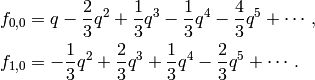
Example 3.29
Next consider  , where we have

The command q_expansion_cuspforms computes
matrices and returns a function
such that  is the -expansion of
 to some precision.
(For efficiency reasons, in Sage actually
computes matrices of acting
on a basis for the linear dual of .)
to some precision.
(For efficiency reasons, in Sage actually
computes matrices of acting
on a basis for the linear dual of .)
sage: M = ModularSymbols(23)
sage: S = M.cuspidal_submodule()
sage: S
Modular Symbols subspace of dimension 4 of Modular
Symbols space of dimension 5 for Gamma_0(23) of weight
2 with sign 0 over Rational Field
sage: f = S.q_expansion_cuspforms(6)
sage: f(0,0)
q - 2/3*q^2 + 1/3*q^3 - 1/3*q^4 - 4/3*q^5 + O(q^6)
sage: f(0,1)
O(q^6)
sage: f(1,0)
-1/3*q^2 + 2/3*q^3 + 1/3*q^4 - 2/3*q^5 + O(q^6)
Thus a basis for  is
is
Or, in echelon form,
which we computed using
sage: S.q_expansion_basis(6)
[
q - q^3 - q^4 + O(q^6),
q^2 - 2*q^3 - q^4 + 2*q^5 + O(q^6)
]
Computing Using Eigenvectors
In this section we describe how to use modular symbols to construct a
basis of consisting of modular forms that are
eigenvectors for every element of the ring  generated by the
Hecke operator , with . Such eigenvectors are called
eigenforms.
generated by the
Hecke operator , with . Such eigenvectors are called
eigenforms.
Suppose is a positive integer that divides . As explained in
[Lan95, VIII.1–2], for each divisor of  there is
a natural degeneracy map
there is
a natural degeneracy map  given by
  . The
new subspace of , denoted
. The
new subspace of , denoted
 , is the complementary -submodule of the
-module generated by the images of all maps
, is the complementary -submodule of the
-module generated by the images of all maps  ,
with and as above. It is a nontrivial fact that this
complement is well defined; one possible proof uses the Petersson
inner product (see [Lan95, Section VII.5]).
,
with and as above. It is a nontrivial fact that this
complement is well defined; one possible proof uses the Petersson
inner product (see [Lan95, Section VII.5]).
The theory of Atkin and Lehner [AL70] (see
Theorem 9.4 below) asserts that, as a -module,
decomposes as follows:
To compute it suffices to compute
 for each
  .
.
We now turn to the problem of computing .
Atkin and Lehner [AL70] proved that
is spanned by eigenforms for all with
and that the common eigenspaces of all the with
each have dimension . Moreover, if  is an eigenform then the coefficient of
in the -expansion of is nonzero, so it is possible to
normalize so the coefficient of is (such a
normalized eigenform in the new subspace is called a
newform). With so normalized, if
is an eigenform then the coefficient of
in the -expansion of is nonzero, so it is possible to
normalize so the coefficient of is (such a
normalized eigenform in the new subspace is called a
newform). With so normalized, if  , then
the
, then
the  Fourier coefficient of is
  . If
. If
 is a normalized eigenvector for all
, then the , with composite, are determined by the
, with prime, by the following formulas:
is a normalized eigenvector for all
, then the , with composite, are determined by the
, with prime, by the following formulas:  when and
  are relatively prime and
  for prime. When
  ,
,
 . We conclude that in order to compute
, it suffices to compute all systems of
eigenvalues
. We conclude that in order to compute
, it suffices to compute all systems of
eigenvalues  of the prime-indexed Hecke
operators
of the prime-indexed Hecke
operators  acting on .
Given a system of eigenvalues, the corresponding eigenform is
, where the , for composite,
are determined by the recurrence given above.
acting on .
Given a system of eigenvalues, the corresponding eigenform is
, where the , for composite,
are determined by the recurrence given above.
In light of the pairing  introduced in
Section Hecke Operators,
computing the above systems of eigenvalues
introduced in
Section Hecke Operators,
computing the above systems of eigenvalues  amounts to computing the systems of eigenvalues of the Hecke operators
on the subspace
amounts to computing the systems of eigenvalues of the Hecke operators
on the subspace  of that corresponds
to the new subspace of
of that corresponds
to the new subspace of  For each proper divisor of and each divisor of
, let
For each proper divisor of and each divisor of
, let  be the map
sending to
be the map
sending to  .
Then is the intersection of the kernels of all
maps
.
Then is the intersection of the kernels of all
maps  .
.
Computing the systems of eigenvalues of a collection of commuting diagonalizable endomorphisms is a problem in linear algebra (see Chapter Linear Algebra).
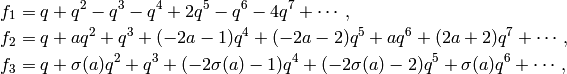
Example 3.30
All forms in are new.
Up to Galois conjugacy, the eigenvalues of the Hecke operators
,  ,
,  , and
, and  on
on  are
are
 and
and  , where
 . Each of these eigenvalues occur
in with multiplicity two; for example,
the characteristic polynomial of on is
. Each of these eigenvalues occur
in with multiplicity two; for example,
the characteristic polynomial of on is
 .
Thus is spanned by
.
Thus is spanned by
where  is the other
  -conjugate of
  .
.
Summary
To compute the -expansion of a basis for , we use
the degeneracy maps so that we only have to solve the problem for
, for all integers . Using modular
symbols, we compute all systems of eigenvalues
 , and then write down the corresponding
eigenforms
, and then write down the corresponding
eigenforms  .
.
Exercises
Exercise 3.1
Suppose that  are in the same orbit for
the action of , i.e., that there exists
are in the same orbit for
the action of , i.e., that there exists
 such that
  . Let
. Let
 and
and  .
Prove that the pairs
.
Prove that the pairs
 and
and
 are
isomorphic.
(By an isomorphism
are
isomorphic.
(By an isomorphism  of pairs, we mean an
isomorphism
of pairs, we mean an
isomorphism  of elliptic curves that sends to
. You may use the fact that an isomorphism of elliptic curves
over is a -linear map
of elliptic curves that sends to
. You may use the fact that an isomorphism of elliptic curves
over is a -linear map  that sends the lattice
corresponding to one curve onto the lattice corresponding to the
other.)
that sends the lattice
corresponding to one curve onto the lattice corresponding to the
other.)
Exercise 3.2
Let  be integers and a positive integer. Prove that the
modular symbol
be integers and a positive integer. Prove that the
modular symbol  is as an element of
. [Hint: See Example 3.6.]
is as an element of
. [Hint: See Example 3.6.]
Exercise 3.3
Let be a prime.
- List representative elements of
 .
. - What is the cardinality of as a function of ?
- Prove that there is a bijection between the right cosets of
 in and the elements of
that sends to . (As mentioned in
this chapter, the analogous statement is also true when the
level is composite; see [Cre97a, Section 2.2] for
complete details.) end{enumerate}
in and the elements of
that sends to . (As mentioned in
this chapter, the analogous statement is also true when the
level is composite; see [Cre97a, Section 2.2] for
complete details.) end{enumerate}
Exercise 3.4
Use the inductive proof of Proposition 3.11 to write
in terms of Manin symbols for  .
.
Exercise 3.5
Show that the Hecke operator acts as multiplication
by on the space  as follows:
- Write down right coset representatives for
 in .
in . - List all eight relations coming from Theorem 3.13.
- Find a single Manin symbols so that the three other
Manin symbols are a nonzero multiple of modulo the
relations found in the previous step.
- Use formula (5) to compute
![T_2([r_i])](_images/math/763be4a6ceaad6949c8165c288985a2bd694aa68.png) . You will
obtain a sum of four symbols. Using the relations above, write
this sum as a multiple of . (The multiple must be or
you made a mistake.)
. You will
obtain a sum of four symbols. Using the relations above, write
this sum as a multiple of . (The multiple must be or
you made a mistake.)