Linear Algebra
This chapter is about several algorithms for matrix algebra over the rational numbers and cyclotomic fields. Algorithms for linear algebra over exact fields are necessary in order to implement the modular symbols algorithms that we will describe in Chapter Linear Algebra. This chapter partly overlaps with [Coh93, Sections 2.1–2.4].
Note: We view all matrices as defining linear transformations by acting on row vectors from the right.
Echelon Forms of Matrices
Definition 7.1
A matrix is in (reduced row) echelon form if each row in the matrix
has more zeros at the beginning than the row above it, the first
nonzero entry of every row is  , and the first nonzero entry of
any row is the only nonzero entry in its column.
, and the first nonzero entry of
any row is the only nonzero entry in its column.
Given a matrix  , there is another matrix
  such that is
obtained from by left multiplication by an invertible matrix
and is in reduced row echelon form. This matrix is called the
echelon form of . It is unique.
such that is
obtained from by left multiplication by an invertible matrix
and is in reduced row echelon form. This matrix is called the
echelon form of . It is unique.
A pivot column of is a column of such that the reduced
row echelon form of contains a leading .
Example 7.2
The following matrix is not in reduced row echelon form:
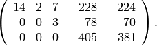
The reduced row echelon form of the above matrix is
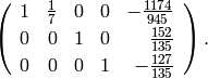
Notice that the entries of the reduced row echelon form can be
rationals with large denominators even though the entries of the
original matrix are integers. Another example is the simple
looking matrix
whose echelon form is
A basic fact is that two matrices and have the same reduced
row echelon form if and only if there is an invertible matrix  such
that
such
that  . Also, many standard operations in linear algebra,
e.g., computation of the kernel of a linear map, intersection of
subspaces, membership checking, etc., can be encoded as a question
about computing the echelon form of a matrix.
. Also, many standard operations in linear algebra,
e.g., computation of the kernel of a linear map, intersection of
subspaces, membership checking, etc., can be encoded as a question
about computing the echelon form of a matrix.
The following standard algorithm computes the echelon form of a matrix.
Algorithm 7.3
Given an  matrix over a field,
the algorithm outputs the reduced row echelon form of .
Write
matrix over a field,
the algorithm outputs the reduced row echelon form of .
Write  for the
  entry of ,
where
entry of ,
where  and
and  .
.
- [Initialize] Set
 .
. - [Clear Each Column] For each column
 ,
clear the
,
clear the  column as follows:
- [First Nonzero] Find the smallest
 such that
 , or if there is no such , go to the next
column.
, or if there is no such , go to the next
column. - [Rescale] Replace row of by
 times row .
 - [Swap] Swap row with row
 .
. - [Clear] For each
 with
with  ,
if
,
if  , add
, add  times row of to
row
times row of to
row  to clear the leading entry of the
  row.
row. - [Increment] Set
 .
.
- [First Nonzero] Find the smallest
This algorithm takes  arithmetic operations in the base field,
where is an matrix. If the base field is
arithmetic operations in the base field,
where is an matrix. If the base field is  , the
entries can become huge and arithmetic operations are then
very expensive. See Section Echelon Forms over for ways
to mitigate this problem.
, the
entries can become huge and arithmetic operations are then
very expensive. See Section Echelon Forms over for ways
to mitigate this problem.
To conclude this section, we mention how to convert a few standard problems into questions about reduced row echelon forms of matrices. Note that one can also phrase some of these answers in terms of the echelon form, which might be easier to compute, or an LUP decomposition (lower triangular times upper triangular times permutation matrix), which the numerical analysts use.
Kernel of
: We explain how to compute the
kernel of acting on column vectors from the right (first
transpose to obtain the kernel of acting on row vectors).
Since passing to the reduced row echelon form of is the same
as multiplying on the left by an invertible matrix, the kernel of
the reduce row echelon form of is the same as the kernel
of . There is a basis vector of  that corresponds to
each nonpivot column of . That vector has a at the
nonpivot column,
that corresponds to
each nonpivot column of . That vector has a at the
nonpivot column,  ‘s at all other nonpivot columns, and for each
pivot column, the negative of the entry of at the nonpivot
column in the row with that pivot element.
‘s at all other nonpivot columns, and for each
pivot column, the negative of the entry of at the nonpivot
column in the row with that pivot element.Intersection of Subspaces: Suppose
 and
and  are subspace
of a finite-dimensional vector space
are subspace
of a finite-dimensional vector space  . Let
. Let  and
and  be
matrices whose columns form a basis for and ,
respectively. Let
be
matrices whose columns form a basis for and ,
respectively. Let ![A=[A_1 | A_2]](_images/math/c04d9d985fe2b413bd3949ade54970579a165913.png) be the augmented matrix formed
from and . Let
be the augmented matrix formed
from and . Let  be the kernel of the linear
transformation defined by . Then is isomorphic to the
desired intersection. To write down the intersection explicitly,
suppose that
be the kernel of the linear
transformation defined by . Then is isomorphic to the
desired intersection. To write down the intersection explicitly,
suppose that  and do the following: For
each
and do the following: For
each  in a basis for , write down the linear combination of a
basis for obtained by taking the first
in a basis for , write down the linear combination of a
basis for obtained by taking the first  entries of
the vector . The fact that is in
entries of
the vector . The fact that is in  implies that the
vector we just wrote down is also in . This is because a
linear relation
implies that the
vector we just wrote down is also in . This is because a
linear relation
i.e., an element of that kernel, is the same as
For more details, see [Coh93, Alg. 2.3.9].
Rational Reconstruction
Rational reconstruction is a process that allows one to sometimes lift
an integer modulo  uniquely to a bounded rational number.
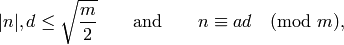
Algorithm 7.4
Given an integer  and an integer
  , this algorithm
computes the numerator
, this algorithm
computes the numerator  and denominator
  of the unique
rational number
of the unique
rational number  , if it exists, with
(1)
or it reports that there is no such number.
- [Reduce mod ] Replace
 with the least integer between
and
with the least integer between
and  that is congruent to modulo .
 - [Trivial Cases] If
 or
or  , return .
item{} [Initialize] Let
, return .
item{} [Initialize] Let  ,
,  ,
,  , and set
 and
and  . Use the notation
  and
and  to refer to the entries of
  , for
, for  .
. - [Iterate] Do the following as long as
 :
Set
:
Set  ,
set
,
set  , and set
  and
and  .
. - [Numerator and Denominator] Set
 and
and  .
. - [Good?] If
 and
and  , return ;
otherwise report that there is no rational number as
in (1).
, return ;
otherwise report that there is no rational number as
in (1).
Algorithm 7.4 for rational reconstruction is described (with proof) in [Knu, pgs. 656–657] as the solution to Exercise 51 on page 379 in that book. See, in particular, the paragraph right in the middle of page 657, which describes the algorithm. Knuth attributes this rational reconstruction algorithm to Wang, Kornerup, and Gregory from around 1983.
We now give an indication of why Algorithm 7.4 computes
the rational reconstruction of  , leaving the precise
details and uniqueness to [Knu, pgs. 656–657]. At each
step in Algorithm 7.4, the
, leaving the precise
details and uniqueness to [Knu, pgs. 656–657]. At each
step in Algorithm 7.4, the  -tuple
  satisfies
(2)
and similarly for  .
When computing the usual extended
.
When computing the usual extended  , at the end
  and
and  ,
,  give a representation of the
  as a
as a  -linear
combination of and .
In Algorithm 7.4, we are instead interested
in finding a rational number such that
-linear
combination of and .
In Algorithm 7.4, we are instead interested
in finding a rational number such that
 . If we set
  and
and  in (2) and rearrange, we obtain
Thus at every step of the algorithm we find a rational number
such that  . The problem at intermediate
steps is that, e.g., could be , or or
could be too large.
. The problem at intermediate
steps is that, e.g., could be , or or
could be too large.
Example 7.5
We compute an example using Sage.
sage: p = 389
sage: k = GF(p)
sage: a = k(7/13); a
210
sage: a.rational_reconstruction()
7/13
Echelon Forms over 
A difficulty with computation of the echelon form of a matrix over the
rational numbers is that arithmetic with large rational numbers is
time-consuming; each addition potentially requires a
and numerous additions and multiplications of integers. Moreover, the
entries of during intermediate steps of Algorithm 7.3
can be huge even though the entries of and the answer are small.
For example, suppose is an invertible square matrix. Then the
echelon form of is the identity matrix, but during intermediate
steps the numbers involved could be quite large. One technique for
mitigating this is to compute the echelon form using a
multimodular method.
If is a matrix with rational entries, let  be the
height of , which is the maximum of the absolute values of
the numerators and denominators of all entries of . If
be the
height of , which is the maximum of the absolute values of
the numerators and denominators of all entries of . If  are
rational numbers and
are
rational numbers and  is a prime, we write
  to
mean that the denominators of
to
mean that the denominators of  and
and  are not divisible by but
the numerator of the rational number
are not divisible by but
the numerator of the rational number  (in reduced form) is
divisible by . For example, if
(in reduced form) is
divisible by . For example, if  and
and  , then
 , so
, so  .
.
Algorithm 7.6
Given an matrix with entries in ,
this algorithm computes the reduced row echelon form of .
Rescale the input matrix
to have integer entries. This does
not change the echelon form and makes reduction modulo many
primes easier. We may thus assume has integer entries.Let
 be a guess for the height of the echelon form.
List successive primes
 such that the product
of the
such that the product
of the  is greater than
  , where
is the number of columns of .
, where
is the number of columns of .Compute the echelon forms
 of the reduction
  using, e.g., Algorithm 7.3 or any other echelon algorithm. %
(This is where most of the work takes place.)
using, e.g., Algorithm 7.3 or any other echelon algorithm. %
(This is where most of the work takes place.)Discard any
whose pivot column list is not maximal among
pivot lists of all  found so far. (The pivot list
associated to is the ordered list of integers such
that the
found so far. (The pivot list
associated to is the ordered list of integers such
that the  column of is a pivot column. We mean
maximal with respect to the following ordering on integer
sequences: shorter integer sequences are smaller, and if two
sequences have the same length, then order in reverse
lexicographic order. Thus
column of is a pivot column. We mean
maximal with respect to the following ordering on integer
sequences: shorter integer sequences are smaller, and if two
sequences have the same length, then order in reverse
lexicographic order. Thus ![[1,2]](_images/math/92bb4c21c8491453be13b7f2d521b1934160031f.png) is smaller than
is smaller than ![[1,2,3]](_images/math/e8dd506f76559bbb9c2095066d6957f810c5e6f4.png) ,
and
,
and ![[1,2,7]](_images/math/c8420c4644c18a2ba96be4cb91c09dafb337dfab.png) is smaller than
is smaller than ![[1,2,5]](_images/math/70945f442c2f9afa027c81f961e7889091d24286.png) . Think of maximal as
“optimal”, i.e., best possible pivot columns.)
. Think of maximal as
“optimal”, i.e., best possible pivot columns.)Use the Chinese Remainder Theorem to find a matrix
with
integer entries such that  for all .
Use Algorithm 7.4 to try to find a matrix
 whose
coefficients are rational numbers
whose
coefficients are rational numbers  such that
 , where
  , and
, and  for each prime . If rational reconstruction fails, compute a
few more echelon forms mod the next few primes (using the above
steps) and attempt rational reconstruction again. Let be
the matrix over so obtained. (A trick here is to keep
track of denominators found so far to avoid doing very many
rational reconstructions.)
for each prime . If rational reconstruction fails, compute a
few more echelon forms mod the next few primes (using the above
steps) and attempt rational reconstruction again. Let be
the matrix over so obtained. (A trick here is to keep
track of denominators found so far to avoid doing very many
rational reconstructions.)Compute the denominator
of , i.e., the smallest positive
integer such that  has integer entries. If
(3)
then
is the reduced row echelon form of . If not,
repeat the above steps with a few more primes.
Proof
We prove that if (3) is satisfied, then the
matrix computed by the algorithm really is the reduced row
echelon form  of . First note that is in reduced row
echelon form since the set of pivot columns of all matrices
used to construct are the same, so the pivot columns of are
the same as those of any and all other entries in the
pivot columns are , so the other entries of in the pivot
columns are also .
of . First note that is in reduced row
echelon form since the set of pivot columns of all matrices
used to construct are the same, so the pivot columns of are
the same as those of any and all other entries in the
pivot columns are , so the other entries of in the pivot
columns are also .
Recall from the end of Section Echelon Forms of Matrices that a matrix
whose columns are a basis for the kernel of can be obtained from
the reduced row echelon form . Let be the matrix whose
columns are the vectors in the kernel algorithm applied to ,
so  . Since the reduced row echelon form is obtained by left
multiplying by an invertible matrix, for each , there is
an invertible matrix mod such that
. Since the reduced row echelon form is obtained by left
multiplying by an invertible matrix, for each , there is
an invertible matrix mod such that  so
so

Since  and are integer matrices, the Chinese
remainder theorem implies that
and are integer matrices, the Chinese
remainder theorem implies that
The integer entries of  all satisfy
 ,
where is the number of columns of . Since
,
where is the number of columns of . Since  ,
the bound (3) implies that
,
the bound (3) implies that  . Thus
 , so
, so  . On the other hand,
the rank of equals the rank of each (since the pivot columns
are the same), so
. On the other hand,
the rank of equals the rank of each (since the pivot columns
are the same), so

Thus  , and combining
this with the bound obtained above, we see that
, and combining
this with the bound obtained above, we see that
 . This implies that is the reduced row
echelon form of , since two matrices have the same kernel if
and only if they have the same reduced row echelon form
(the echelon form is an invariant of the row space, and the
kernel is the orthogonal complement of the row space).
. This implies that is the reduced row
echelon form of , since two matrices have the same kernel if
and only if they have the same reduced row echelon form
(the echelon form is an invariant of the row space, and the
kernel is the orthogonal complement of the row space).
The reason for step (5) is that the matrices need
not be the reduction of modulo , and indeed this
reduction might not even be defined, e.g., if divides the
denominator of some element of , then this reduction makes no
sense. For example, set  and suppose
  .
Then
.
Then  , which has no reduction modulo ; also,
the reduction of modulo is
, which has no reduction modulo ; also,
the reduction of modulo is  , which is already in reduced row echelon form. However if
we were to combine with the echelon form of modulo another
prime, the result could never be lifted using rational reconstruction.
Thus the reason we exclude all with nonmaximal pivot column
sequence is so that a rational reconstruction will exist. There are
only finitely many primes that divide denominators of entries of ,
so eventually all will have maximal pivot column sequences,
i.e., they are the reduction of the true reduced row echelon form , so
the algorithm terminates.
, which is already in reduced row echelon form. However if
we were to combine with the echelon form of modulo another
prime, the result could never be lifted using rational reconstruction.
Thus the reason we exclude all with nonmaximal pivot column
sequence is so that a rational reconstruction will exist. There are
only finitely many primes that divide denominators of entries of ,
so eventually all will have maximal pivot column sequences,
i.e., they are the reduction of the true reduced row echelon form , so
the algorithm terminates.
Remark 7.7
Algorithm 7.6, with sparse matrices seems to
work very well in practice. A simple but helpful
modification to Algorithm 7.3 in the sparse case is to
clear each column using a row with a minimal number of nonzero
entries, so as to reduce the amount of “fill in” (denseness) of
the matrix. There are much more sophisticated methods along these
lines called “intelligent Gauss elimination”. (Cryptographers are
interested in linear algebra mod with huge sparse matrices,
since they come up in attacks on the discrete log problem and
integer factorization.)
One can adapt Algorithm 7.6 to computation of
echelon forms of matrices over cyclotomic fields  .
Assume has denominator . Let be a prime that splits
completely in . Compute the homomorphisms
.
Assume has denominator . Let be a prime that splits
completely in . Compute the homomorphisms
![f_i : \Z_p[\zeta_n] \to \F_p](_images/math/2e4bbd1e593ad956016d56e9d131ff5a24adf7d5.png) by finding the elements of order in
by finding the elements of order in
 . Then compute the mod matrix
  for each , and
find its reduced row echelon form. Taken together, the maps
for each , and
find its reduced row echelon form. Taken together, the maps  together induce an isomorphism
 ![\Psi:\F_p[X]/\Phi_n(X) \isom \F_p^d](_images/math/8450552c7c3c087b1c6b732ff780a52af265832d.png) ,
where
,
where  is the
  cyclotomic polynomial and is its
degree. It is easy to compute
cyclotomic polynomial and is its
degree. It is easy to compute  by evaluating
  at
each element of order in
at
each element of order in  . To compute
  , simply
use linear algebra over to invert a matrix that represents
, simply
use linear algebra over to invert a matrix that represents
 . Use to compute the reduced row echelon form of
 , where
  is the nonprime ideal in
 ![\Z[\zeta_n]](_images/math/a51ab57040f45871738bba73241297da2d3f3ce7.png) generated by . Do this for several primes , and use rational
reconstruction on each coefficient of each power of
generated by . Do this for several primes , and use rational
reconstruction on each coefficient of each power of  , to
recover the echelon form of .
, to
recover the echelon form of .
Echelon Forms via Matrix Multiplication
In this section we explain
how to compute echelon forms using matrix multiplication. This is
valuable because there are asymptotically fast, i.e., better than
 field operations, algorithms for matrix multiplication, and
implementations of linear algebra libraries often include
highly optimized matrix multiplication algorithms.
We only sketch the basic ideas
behind these asymptotically fast algorithms (following [Ste]), since more
detail would take us too far from modular forms.
field operations, algorithms for matrix multiplication, and
implementations of linear algebra libraries often include
highly optimized matrix multiplication algorithms.
We only sketch the basic ideas
behind these asymptotically fast algorithms (following [Ste]), since more
detail would take us too far from modular forms.
The naive algorithm for multiplying two  matrices requires
 arithmetic operations in the base ring. In
[Str69], Strassen described a clever algorithm that
computes the product of two matrices in
arithmetic operations in the base ring. In
[Str69], Strassen described a clever algorithm that
computes the product of two matrices in 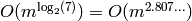 arithmetic operations in the base ring. Because
of numerical stability issues, Strassen’s algorithm is rarely used in
numerical analysis. But for matrix arithmetic over exact base rings
(e.g., the rational numbers, finite fields, etc.) it is of extreme
importance.
arithmetic operations in the base ring. Because
of numerical stability issues, Strassen’s algorithm is rarely used in
numerical analysis. But for matrix arithmetic over exact base rings
(e.g., the rational numbers, finite fields, etc.) it is of extreme
importance.
In [Str69], Strassen also sketched a new algorithm for
computing the inverse of a square matrix using matrix multiplication.
Using this algorithm, the number of operations to invert an
matrix is (roughly) the same as the number needed to multiply two
matrices.
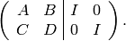
Suppose the input matrix is  and we
write it in block form as
and we
write it in block form as  where
where  are all
 matrices. Assume that any intermediate
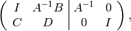
matrices below that we invert are invertible. Consider the augmented
matrix
matrices. Assume that any intermediate
matrices below that we invert are invertible. Consider the augmented
matrix
Multiply the top row by  to obtain
and write  .
Subtract times the first row from the second row to get
.
Subtract times the first row from the second row to get
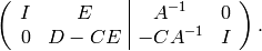
Set 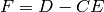 and multiply
the bottom row by
and multiply
the bottom row by  on the left to obtain
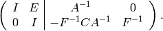
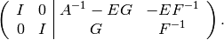
Set 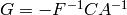 , and subtract
times the second from the first row to
arrive at
, and subtract
times the second from the first row to
arrive at
The idea listed above can, with significant work, be extended to a general algorithm (as is done in [Ste06]).
Next we very briefly sketch how to compute echelon forms of matrices using matrix multiplication and inversion. Its complexity is comparable to the complexity of matrix multiplication.
As motivation, recall the standard algorithm from undergraduate linear
algebra for inverting an invertible square matrix : form the
augmented matrix ![[A|I]](_images/math/1e8da60a7579a29f7560860be44b69ffb45a3d7d.png) , and then compute the echelon form of this
matrix, which is
, and then compute the echelon form of this
matrix, which is ![[I|A^{-1}]](_images/math/6ce82166c1225c94c1c2499e57399dc59b7cd2c5.png) . If
. If  is the transformation matrix to
echelon form, then
is the transformation matrix to
echelon form, then ![T[A|I] = [I|T]](_images/math/231a23c28054f49699b81ce7aff1be46d23e0596.png) , so
, so  . In particular, we
could find the echelon form of by multiplying on the left by
. Likewise, for any matrix with the same number of rows
as , we could find the echelon form of
. In particular, we
could find the echelon form of by multiplying on the left by
. Likewise, for any matrix with the same number of rows
as , we could find the echelon form of ![[A|B]](_images/math/bf14e657075e8443b1bccb621f1526785ddb27ae.png) by multiplying on
the left by . Next we extend this idea to give
an algorithm to compute echelon forms using only matrix multiplication (and
echelon form modulo one prime).
by multiplying on
the left by . Next we extend this idea to give
an algorithm to compute echelon forms using only matrix multiplication (and
echelon form modulo one prime).
Algorithm 7.8
Given a matrix over the rational numbers (or a number field),
this algorithm computes the echelon form of .
1. [Find Pivots] Choose a random prime (coprime to the
denominator of any entry of ) and compute the echelon form of
, e.g., using Algorithm 7.3. Let  be the pivot columns of . When computing the
echelon form, save the positions
be the pivot columns of . When computing the
echelon form, save the positions  of the rows
used to clear each column.
of the rows
used to clear each column.
- [Extract Submatrix] Extract the
 submatrix of
whose entries are
submatrix of
whose entries are  for
for  .
. - [Compute Inverse] Compute the inverse
 of . Note
that must be invertible since its reduction modulo is
invertible.
of . Note
that must be invertible since its reduction modulo is
invertible. - [Multiply] Let be the matrix whose rows are the rows
of . Compute
 . If is
not in echelon form, go to ste (1).
. If is
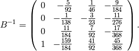
not in echelon form, go to ste (1). - [Done?] Write down a matrix
 whose columns are a basis for
as explained in the Kernel Algorithm. Let
whose columns are a basis for
as explained in the Kernel Algorithm. Let  be
the matrix whose rows are the rows of other than rows
. Compute the product
be
the matrix whose rows are the rows of other than rows
. Compute the product  . If
. If  ,
output , which is the echelon form of . If
,
output , which is the echelon form of . If  , go
to step (1)) and run the whole algorithm
again.
, go
to step (1)) and run the whole algorithm
again.
Proof
We prove both that the algorithm terminates and that when it
terminates, the matrix is the echelon form of .
First we prove that the algorithm terminates. Let be the
echelon form of .
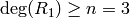
By Exercise 7.3,
for all but finitely many primes (i.e., any
prime where has the same rank as ) the echelon form of
equals  . For any such prime the pivot
columns of are the pivot columns of , so the
algorithm will terminate for that choice of .
. For any such prime the pivot
columns of are the pivot columns of , so the
algorithm will terminate for that choice of .
We next prove that when the algorithm terminates, is the
echelon form of . By assumption, is in echelon form and is
obtained by multiplying on the left by an invertible matrix,
so must be the echelon form of . The rows of are a
subset of those of , so the rows of are a subset of the rows
of the echelon form of . Thus 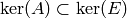 . To
show that equals the echelon form of , we just need to verify
that
. To
show that equals the echelon form of , we just need to verify
that 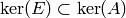 , i.e., that
  , where is as in
step (5). Since is the echelon form of , we
know that
, where is as in
step (5). Since is the echelon form of , we
know that  . By step (5) we also know that
. Thus , since the rows of are the union of the
rows of and .
. By step (5) we also know that
. Thus , since the rows of are the union of the
rows of and .
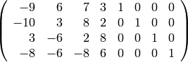
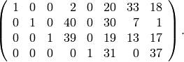
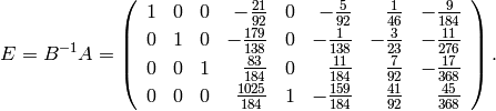
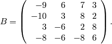
Example 7.9
Let be the  matrix
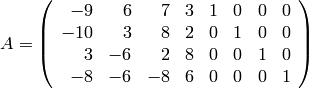
from Example 7.2.
sage: M = MatrixSpace(QQ,4,8)
sage: A = M([[-9,6,7,3,1,0,0,0],[-10,3,8,2,0,1,0,0],
[3,-6,2,8,0,0,1,0],[-8,-6,-8,6,0,0,0,1]])
First choose the “random” prime  , which does not
divide any of the entries of , and compute the
echelon form of the reduction of modulo
, which does not
divide any of the entries of , and compute the
echelon form of the reduction of modulo  .
.
sage: A41 = MatrixSpace(GF(41),4,8)(A)
sage: E41 = A41.echelon_form()
The echelon form of  is
is
Thus we take  ,
,  ,
,  , and
, and  .
Also
.
Also  for
for  .
Next extract the submatrix .
.
Next extract the submatrix .
sage: B = A.matrix_from_columns([0,1,2,4])
The submatrix is
The inverse of is
Multiplying by yields
sage: E = B^(-1)*A
This is not the echelon form of . Indeed, it is not
even in echelon form, since the last row is not
normalized so the leftmost nonzero entry is .
We thus choose another random prime, say  .
The echelon form mod
.
The echelon form mod  has columns
  as pivot columns.
We thus extract the matrix
as pivot columns.
We thus extract the matrix
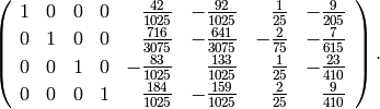
sage: B = A.matrix_from_columns([0,1,2,3])
This matrix has inverse
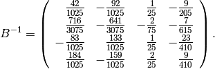
Finally, the echelon form of is  No further
checking is needed since the product so obtained is in echelon
form, and the matrix of the last step of the algorithm has
rows.
No further
checking is needed since the product so obtained is in echelon
form, and the matrix of the last step of the algorithm has
rows.
Remark 7.10
Above we have given only the barest sketch of asymptotically fast “block” algorithms for linear algebra. For optimized algorithms that work in the general case, please see the source code of [Ste06].
Decomposing Spaces under the Action of Matrix
Efficiently solving the following problem is a crucial step in computing a basis of eigenforms for a space of modular forms (see Sections Computing Using Eigenvectors and Newforms: Systems of Eigenvalues).
Problem 7.11
Suppose is an matrix with entries in a field
(typically a number field or finite field) and that the minimal
polynomial of is square-free and has degree . View as
acting on  . Find a simple module decomposition
  of as a direct sum of simple
 ![K[T]](_images/math/7619d30d16974a3af86a1e8c76839bbba3370b99.png) -modules.
Equivalently, find an invertible matrix such that
-modules.
Equivalently, find an invertible matrix such that  is a block direct sum of matrices
  such that the
minimal polynomial of each
such that the
minimal polynomial of each  is irreducible.
Remark 7.12
A generalization of Problem 7.11
to arbitrary matrices with entries in is
finding the rational Jordan form (or rational canonical
form, or Frobenius form) of .
This is like the usual Jordan form, but the resulting matrix is
over and the summands of the matrix corresponding to
eigenvalues are replaced by matrices whose minimal polynomials
are the minimal polynomials (over ) of the eigenvalues. The
rational Jordan form was extensively studied by Giesbrecht in his
Ph.D. thesis and many successive papers, where he analyzes the
complexity of his algorithms and observes that the limiting step is
factoring polynomials over . The reason is that given a polynomial
![f\in K[x]](_images/math/039f104206d80a9cd87a7e60701edff251773932.png) , one can easily write down a matrix such that one can
read off the factorization of
, one can easily write down a matrix such that one can
read off the factorization of  from the rational Jordan form of
(see also [Ste97]).
from the rational Jordan form of
(see also [Ste97]).
Characteristic Polynomials
The computation of characteristic polynomials of matrices is crucial to
modular forms computations. There are many approaches to this
problems: compute  symbolically (bad), compute the traces
of the powers of (bad), or compute the Hessenberg form modulo many
primes and use CRT (bad; see for [Coh93, Section 2.2.4] the
definition of Hessenberg form and the algorithm). A more
sophisticated method is to compute the rational canonical form of
using Giesbrecht’s algorithm [1] (see [GS02]),
which involves computing Krylov subspaces
(see Remark Remark 7.13 below), and building up the whole
space on which acts. This latter method is a generalization of
Wiedemann’s algorithm for computing minimal polynomials (see
Section Wiedemann’s Minimal Polynomial Algorithm), but with more structure to handle the
case when the characteristic polynomial is not equal to the minimal
polynomial.
symbolically (bad), compute the traces
of the powers of (bad), or compute the Hessenberg form modulo many
primes and use CRT (bad; see for [Coh93, Section 2.2.4] the
definition of Hessenberg form and the algorithm). A more
sophisticated method is to compute the rational canonical form of
using Giesbrecht’s algorithm [1] (see [GS02]),
which involves computing Krylov subspaces
(see Remark Remark 7.13 below), and building up the whole
space on which acts. This latter method is a generalization of
Wiedemann’s algorithm for computing minimal polynomials (see
Section Wiedemann’s Minimal Polynomial Algorithm), but with more structure to handle the
case when the characteristic polynomial is not equal to the minimal
polynomial.
Polynomial Factorization
Factorization of polynomials in ![\Q[X]](_images/math/175755dc07dfb52becffdc117a4590a8d3970ac4.png) (or over number fields) is an
important step in computing an explicit basis of Hecke eigenforms for
spaces of modular forms. The best algorithm is the van Hoeij method
[BHKS06],
which uses the LLL lattice basis reduction algorithm [LLL82] in a
novel way to solve the optimization problems that come up in trying to
lift factorizations mod to .
It has been generalized by Belebas, van Hoeij, Kl”uners, and Steel
to number fields.
(or over number fields) is an
important step in computing an explicit basis of Hecke eigenforms for
spaces of modular forms. The best algorithm is the van Hoeij method
[BHKS06],
which uses the LLL lattice basis reduction algorithm [LLL82] in a
novel way to solve the optimization problems that come up in trying to
lift factorizations mod to .
It has been generalized by Belebas, van Hoeij, Kl”uners, and Steel
to number fields.
Wiedemann’s Minimal Polynomial Algorithm
In this section we describe
an algorithm due to Wiedemann for computing the
minimal polynomial of an matrix over a field.
Choose a random vector  and compute the iterates
(4)
If  is the minimal polynomial of , then

where  is the identity matrix.
For any
is the identity matrix.
For any  , by
multiplying both sides on the right by the vector
, by
multiplying both sides on the right by the vector  , we see that

hence

Wiedemann’s idea is to observe that any single component of the
vectors  satisfies the linear recurrence with
coefficients
satisfies the linear recurrence with
coefficients  . The Berlekamp-Massey
algorithm (see Algorithm 7.14 below) was introduced in the
1960s in the context of coding theory to find the minimal polynomial
of a linear recurrence sequence
. The Berlekamp-Massey
algorithm (see Algorithm 7.14 below) was introduced in the
1960s in the context of coding theory to find the minimal polynomial
of a linear recurrence sequence  . The minimal polynomial of
this linear recurrence is by definition the unique monic
polynomial
. The minimal polynomial of
this linear recurrence is by definition the unique monic
polynomial  , such that if satisfies a linear recurrence
 (for all
  ), then divides the polynomial
  .
If we apply Berlekamp-Massey to the top coordinates of the
.
If we apply Berlekamp-Massey to the top coordinates of the  , we
obtain a polynomial
, we
obtain a polynomial  , which divides . We then apply it to the
second to the top coordinates and find a polynomial
, which divides . We then apply it to the
second to the top coordinates and find a polynomial  that
divides , etc. Taking the least common multiple of the first few
that
divides , etc. Taking the least common multiple of the first few  , we
find a divisor of the minimal polynomial of . One can show that
with “high probability” one quickly finds , instead of just a
proper divisor of .
, we
find a divisor of the minimal polynomial of . One can show that
with “high probability” one quickly finds , instead of just a
proper divisor of .
Remark 7.13
In the literature, techniques that involve iterating a vector as in (4) are often called Krylov methods. The subspace generated by the iterates of a vector under a matrix is called a Krylov subspace.
Algorithm 7.14
Suppose  are the first
  terms of a
sequence that satisfies a linear recurrence of degree at most .
This algorithm computes the minimal
polynomial of the sequence.
terms of a
sequence that satisfies a linear recurrence of degree at most .
This algorithm computes the minimal
polynomial of the sequence.
- Let
 ,
,  ,
,
 ,
,  .
. - While
 , do the following:
- Compute
 and such that
  .
. - Let
 .
.
- Compute
- Let
 and set
 .
. - Let be the leading coefficient of
 and output
 .
.
The above description of Berlekamp-Massey is taken from [AD04], which contains some additional ideas for improvements.
Now suppose is an matrix as in
Problem Problem 7.11. We find the minimal polynomial of by
computing the minimal polynomial of  using Wiedemann’s
algorithm, for many primes , and using the Chinese Remainder
Theorem. (One has to bound the number of primes that must be
considered; see, e.g., [Coh93].)
using Wiedemann’s
algorithm, for many primes , and using the Chinese Remainder
Theorem. (One has to bound the number of primes that must be
considered; see, e.g., [Coh93].)
One can also compute the characteristic polynomial of directly
from the Hessenberg form of , which can be computed in  field operations, as described in [Coh93]. This is
simple but slow. Also, the we consider will often be sparse,
and Wiedemann is particularly good when is sparse.
field operations, as described in [Coh93]. This is
simple but slow. Also, the we consider will often be sparse,
and Wiedemann is particularly good when is sparse.
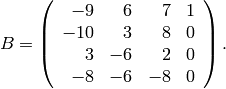
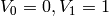
Example 7.15
We compute the minimal polynomial of
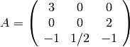
using Wiedemann’s algorithm. Let  . Then

The linear recurrence sequence coming from the first entries is
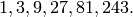
This sequence satisfies the linear recurrence

so its minimal polynomial is  . This implies that
divides the minimal polynomial of the matrix .
Next we use the sequence of second coordinates of the
iterates of , which is
. This implies that
divides the minimal polynomial of the matrix .
Next we use the sequence of second coordinates of the
iterates of , which is

The recurrence that this sequence satisfies is slightly
less obvious, so we apply the Berlekamp-Massey algorithm
to find it, with  .
.
We have
 ,
, 
 .
.Dividing
 by
by  , we find
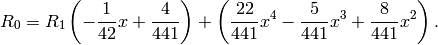
The new
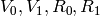 are
are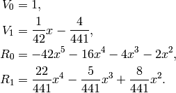
Since
 , we do the above three steps again.
We repeat the above three steps.
Dividing
by , we find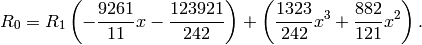
The new
are: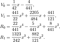
We have to repeat the steps yet again:
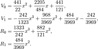
We have
 ,
so
,
so  .
.Multiply through by
 and output
The minimal polynomial of  is
is  ,
since the minimal polynomial has degree at most
and is divisible by .
,
since the minimal polynomial has degree at most
and is divisible by .
-adic Nullspace
We will use the following algorithm of Dixon [Dix82] to
compute -adic approximations to solutions of linear equations
over . Rational reconstruction modulo  then allows us
to recover the corresponding solutions over .
then allows us
to recover the corresponding solutions over .
Algorithm 7.16
Given a matrix with integer entries and nonzero kernel, this
algorithm computes a nonzero element of  using successive -adic approximations.
[Prime] Choose a random prime
.[Echelon] Compute the echelon form of
modulo .[Done?] If
has full rank modulo , it has full rank,
so we terminate the algorithm.[Setup] Let
 .
.[Iterate] For each
 , use the echelon form of
modulo to find a vector
, use the echelon form of
modulo to find a vector  with integer entries such
that
with integer entries such
that  , and then set
(If
 , choose
  .)
.)[
-adic Solution]
Let  .
.[Lift] Use rational reconstruction (Algorithm 7.4) to find a vector
 with rational entries such that
 , if such a vector exists. If the vector does
not exist, increase or use a different . Otherwise,
output .
, if such a vector exists. If the vector does
not exist, increase or use a different . Otherwise,
output .
Proof
We verify the case  only.
We have
only.
We have  and
and  .
Thus
.
Thus

Decomposition Using Kernels
We now know enough to give an algorithm to solve Problem Problem 7.11.
Algorithm 7.17
Given an matrix over a field as
in Problem 7.11,
this algorithm computes the
decomposition of as a direct sum of
simple modules.
- [Minimal Polynomial] Compute the minimal polynomial of ,
e.g., using the multimodular Wiedemann algorithm.
- [Factorization] Factor using the
algorithm in Section Polynomial Factorization.
- [Compute Kernels]
For each irreducible factor of , compute
the following.
- Compute the matrix
 .
. - Compute
 , e.g., using Algorithm 7.16.
- Compute the matrix
- [Output Answer] Then
 .
.
Remark 7.18
As mentioned in Remark Remark 7.12,
if one can compute such decompositions , then
one can easily factor polynomials ; hence the difficulty of
polynomial factorization
is a lower bound on the complexity of writing
as a direct sum of simples.
Exercises
Exercise 7.1
Given a subspace  of
of  , where is a field and
 is an integer, give an algorithm to find
a matrix such that
is an integer, give an algorithm to find
a matrix such that  .
.
Exercise 7.2
If  denotes the row reduced echelon form of
and is a prime not dividing any denominator
of any entry of or of , is
denotes the row reduced echelon form of
and is a prime not dividing any denominator
of any entry of or of , is
 ?
?
Exercise 7.3
Let be a matrix with entries in . Prove that
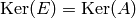
for all but finitely many primes we have
.
Exercise 7.4
Let
- Compute the echelon form of
using each of Algorithm 7.3, Algorithm 7.6,
and Algorithm 7.8.
- Compute the kernel of .
- Find the characteristic polynomial of
using the algorithm of Section Wiedemann’s Minimal Polynomial Algorithm.
Exercise 7.5
The notion of echelon form extends to matrices whose entries come
from certain rings other than fields, e.g., Euclidean domains. In
the case of matrices over we define a matrix to be in echelon
form (or Hermite normal form) if it satisfies
 , for
, for  ,
, ,
, for all
  (unless
  , in which case all ).
There are algorithms for computing with finitely generated
modules over that are analogous to the ones in this chapter
for vector spaces, which depend on computation of Hermite
forms.
- Show that the Hermite form of
 is
is
 .
. - Describe an algorithm for transforming
an matrix with integer entries
into Hermite form using row
operations and the Euclidean algorithm.
Footnotes
| [1] | Allan Steel also invented a similar algorithm. |