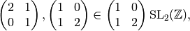
General Modular Symbols
In this chapter we explain how to generalize the notion of modular symbols given in Chapter Modular Forms of Weight 2 to higher weight and more general level. We define Hecke operators on them and their relation to modular forms via the integration pairing. We omit many difficult proofs that modular symbols have certain properties and instead focus on how to compute with modular symbols. For more details see the references given in this section (especially [Mer94]) and [Wie05].
Modular symbols are a formalism that make it
elementary to compute with homology or cohomology related to certain
Kuga-Sato varieties (these are  ,
where
,
where  is a modular curve and
  is the universal elliptic curve
over it). It is not necessary to know anything about these Kuga-Sato
varieties in order to compute with modular symbols.
is the universal elliptic curve
over it). It is not necessary to know anything about these Kuga-Sato
varieties in order to compute with modular symbols.
This chapter is about spaces of modular symbols and how to compute with them. It is by far the most important chapter in this book. The algorithms that build on the theory in this chapter are central to all the computations we will do later in the book.
This chapter closely follows Lo”{i}c Merel’s paper [Mer94].
First we define modular symbols of weight  . Then we define
the corresponding Manin symbols and state a theorem of
Merel-Shokurov, which gives all relations between Manin symbols. (The
proof of the Merel-Shokurov theorem is beyond the scope of this book
but is presented nicely in [Wie05].)
Next we describe how the Hecke operators act on both modular and Manin
symbols and how to compute trace and inclusion maps between spaces of
modular symbols of different levels.
. Then we define
the corresponding Manin symbols and state a theorem of
Merel-Shokurov, which gives all relations between Manin symbols. (The
proof of the Merel-Shokurov theorem is beyond the scope of this book
but is presented nicely in [Wie05].)
Next we describe how the Hecke operators act on both modular and Manin
symbols and how to compute trace and inclusion maps between spaces of
modular symbols of different levels.
Not only are modular symbols useful for computation, but they have
been used to prove theoretical results about modular forms. For
example, certain technical calculations with modular symbols are used
in Lo”{i}c Merel’s proof of the uniform boundedness conjecture for
torsion points on elliptic curves over number fields (modular symbols
are used to understand linear independence of Hecke
operators). Another example is [Gri05], which
distills hypotheses about Kato’s Euler system in  of modular
curves to a simple formula involving modular symbols (when the
hypotheses are satisfied, one obtains a lower bound on the
Shafarevich-Tate group of an elliptic curve).
of modular
curves to a simple formula involving modular symbols (when the
hypotheses are satisfied, one obtains a lower bound on the
Shafarevich-Tate group of an elliptic curve).
Modular Symbols
We recall from Chapter Modular Forms of Weight 2
the free abelian group  of modular symbols.
We view these as elements of the relative
homology of the extended upper half plane
of modular symbols.
We view these as elements of the relative
homology of the extended upper half plane
 relative to the cusps.
The group
is the free abelian group on symbols
relative to the cusps.
The group
is the free abelian group on symbols  with
with
modulo the relations

for all  , and all torsion.
More precisely,
, and all torsion.
More precisely,
where  is the free abelian group on all pairs
 and
and  is the subgroup generated by all elements of
the form
is the subgroup generated by all elements of
the form  .
Note that is a huge free abelian group of countable rank.
.
Note that is a huge free abelian group of countable rank.
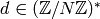
For any integer  , let
, let
![\Z[X,Y]_n](_images/math/5b9e60a40ec8663f7ade0ab999dac4a8a83352eb.png) be the abelian group of homogeneous polynomials of
degree
be the abelian group of homogeneous polynomials of
degree  in two variables
  .
.
Remark 1.22
Note that is isomorphic
to  as a group, but certain natural actions are
different. In [Mer94], Merel
uses the notation
as a group, but certain natural actions are
different. In [Mer94], Merel
uses the notation ![\Z_{n}[X,Y]](_images/math/f5bd5b52ff6e9e94a97a9dd9f1644bde2ae4c4b3.png) for what we
denote by
for what we
denote by ![\Z[X,Y]_{n}](_images/math/230c3f9b9c9bf2e49ccc6721a3faa1f02ff74844.png) .
.
Now fix an integer . Set
![\sM_k = \Z[X,Y]_{k-2} \tensor_\Z \sM_2,](_images/math/a8bfb4b22fc3e9022b856cb38e896c916c057b2c.png)
which is a torsion-free abelian group whose elements are
sums of expressions of the form  .
For example,
.
For example,

Fix a finite index subgroup  of
of  .
Define a left action of on
.
Define a left action of on ![\Z[X,Y]_{k-2}](_images/math/a9324272819ac453b8e5c0ca3d0c8ec01cf8a577.png) as follows. If
as follows. If
 and
and ![P(X,Y)\in \Z[X,Y]_{k-2}](_images/math/e44be5318548c58384d0c35ce502fc54e1316300.png) , let
, let

Note that if we think of  as a column vector, then
since  . The reason
for the inverse is so that this is a left action instead of a right
action, e.g., if
. The reason
for the inverse is so that this is a left action instead of a right
action, e.g., if  , then

Recall that we let act on the left on by
where acts via linear fractional transformations,
so if  , then
For example, useful special cases to remember are that if , then
(Here we view  as
as  in order to describe the
action.)
in order to describe the
action.)
We now combine these two actions to obtain a left action of on  ,
which is given by
,
which is given by

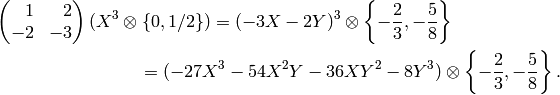
For example,
We will often write
 for
for 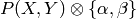 .
.
Definition 1.23
Let be an integer and let be a finite index subgroup of .
The space  of weight
  modular symbols for is the quotient of
 by all relations
  for
for  ,
,  , and by any torsion.
Note that is a torsion-free abelian group, and it is a
nontrivial fact that has finite rank. We denote modular
symbols for in exactly the same way we denote elements of ;
the group will be clear from context.
The space of modular symbols over a ring is

Manin Symbols
Let be a finite index subgroup of and
an integer.
Just as in Chapter Modular Forms of Weight 2 it is possible to compute
using a computer, despite that, as defined above,
is the quotient of one infinitely generated abelian group
by another one. This section is about Manin symbols, which are a
distinguished subset of that lead to a finite presentation
for . Formulas written in terms of Manin symbols are
frequently much easier to compute using a computer than formulas in
terms of modular symbols.
Suppose ![P\in \Z[X,Y]_{k-2}](_images/math/c004809fdb93273e52b7dcf7cd42a6c477a8a83a.png) and
and  .
Then the Manin symbol associated to this
pair of elements is
.
Then the Manin symbol associated to this
pair of elements is
![[P,g] = g(P\{0,\infty\}) \in \sM_k(G).](_images/math/63419a634500f48284f39fd6e421ea3b39886b4f.png)
Notice that if  , then
 ![[P,g] = [P,h]](_images/math/64aae1059073aa276241f2852d1099a4fcac5c60.png) , since
the symbol
, since
the symbol  is invariant
by the action of on the left (by definition,
since it is a modular symbol for ).
Thus for a right coset
is invariant
by the action of on the left (by definition,
since it is a modular symbol for ).
Thus for a right coset  it makes sense to
write
it makes sense to
write ![[P, Gg]](_images/math/21959b833d682c8d2983050da44f60298f63be76.png) for the symbol
for the symbol ![[P,h]](_images/math/221b615b82a0f46a99cc90e371f8a3c711cdd914.png) for any
for any  .
Since has finite index in ,
the abelian group generated by Manin symbols is of finite rank, generated by
.
Since has finite index in ,
the abelian group generated by Manin symbols is of finite rank, generated by
![\bigl\{ [X^{k-2-i}Y^i, \, Gg_j] \, : \, i = 0,\ldots, k-2 \quad\text{and}\quad j = 0,\ldots, r \bigr\},](_images/math/dfe25a6139bec3bf7dc69abd111bc489692047c1.png)
where  run through representatives for the
right cosets
run through representatives for the
right cosets  .
.
We next show that every modular symbol can be written as
a  -linear combination of Manin symbols,
so they generate .
-linear combination of Manin symbols,
so they generate .
Proposition 1.24
The Manin symbols generate .
Proof
The proof if very similar to that
of Proposition 3.11 except we introduce an
extra twist to deal with the polynomial part.
Suppose that we are given a modular
symbol  and wish to represent it as a
sum of Manin symbols. Because
and wish to represent it as a
sum of Manin symbols. Because

it suffices to write  in
terms of Manin symbols.
Let
in
terms of Manin symbols.
Let

denote the continued fraction convergents of the
rational number  .
Then
.
Then

If we let
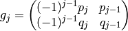 ,
then
,
then  and
and
![P\{0,a/b\}
&=P\sum_{j=-1}^{r}\left\{\frac{p_{j-1}}{q_{j-1}},\frac{p_j}{q_j}\right\}\\
&=\sum_{j=-1}^{r} g_j((g_j^{-1}P)\{0,\infty\})\\
&=\sum_{j=-1}^{r} [g_j^{-1}P,\,\,g_j].](_images/math/2e266b2845256cb60a16d1fc51567dd4b4991219.png)
Since and  has integer coefficients,
the polynomial
has integer coefficients,
the polynomial  also has integer coefficients,
so we introduce no denominators.
also has integer coefficients,
so we introduce no denominators.
Now that we know the Manin symbols generate , we
next consider the relations between Manin symbols. Fortunately,
the answer is fairly simple (though the proof is not). Let
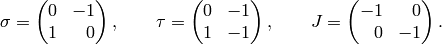
Define a right action of on Manin symbols
as follows. If  , let
, let
![[P, g]h = [h^{-1} P, gh].](_images/math/a8e843b922349d137fc6063fd055e68bb39dead9.png)
This is a right action because both  and
and  are right actions.
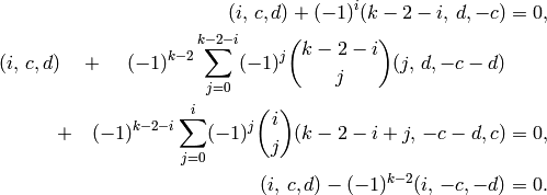
Theorem 1.25
If  is a Manin symbol, then
Moreover, these are all the relations between Manin symbols, in the
sense that the space of modular symbols is isomorphic to
the quotient of the free abelian group on the finitely many symbols
![[X^{i}Y^{k-2-i},Gg]](_images/math/3aff7d2fef9fdb1d42dd4728904be62bf7ce4415.png) (for
(for  and
and
 ) by the above relations and any torsion.
Proof
First we prove that the Manin symbols satisfy the above relations. We follow Merel’s proof (see [Mer94, Section 1.2]). Note that

Writing ![x=[P,g]](_images/math/6b3803bc751eec0dfc102607a5790dba0838aa92.png) , we have
, we have
![[P,g] + [P,g]\sigma &=
[P,g] + [\sigma^{-1}P, g\sigma]\\
&= g(P\{0,\infty\}) + g\sigma (\sigma^{-1}P \{0,\infty\})\\
&=
(gP) \{ g(0), g(\infty) \} +
(g\sigma)(\sigma^{-1} P)\{ g\sigma(0), g\sigma(\infty)\} \\
&= (gP) \{ g(0), g(\infty) \} +
(gP)\{ g(\infty), g(0)\} \\
&= (gP)\{ g(0), g(\infty) \} + \{ g(\infty), g(0)\})\\
&= 0.](_images/math/fb61f47065c6df67ac3052f5978677163216a51a.png)
Also,
![[P,g] &+ [P,g]\tau + [P,g]\tau^2 =
[P,g] + [\tau^{-1}P, g\tau] + [\tau^{-2}P, g\tau^2]\\
&=
g(P\{0,\infty\}) +
g\tau(\tau^{-1}P \{0,\infty\})
+ g\tau^2(\tau^{-2}P \{0,\infty\}) \\
&= (gP) \{ g(0), g(\infty) \} +
(gP) \{ g \tau(0),g\tau(\infty)\}
+ (gP) \{ g\tau^2(0),\tau^2(\infty)\} \\
&= (gP) \{ g(0), g(\infty) \} +
(gP) \{ g(1),g(0)\})
+ (gP) \{ g(\infty), g(1)\} \\
&= (gP)\bigl(\{ g(0), g(\infty)\} +
\{ g(\infty), g(1)\} + \{ g(1),g(0)\}\bigr) \\
&= 0.](_images/math/31e598c5ae7d78904859b94dbcab66a1a01fbdf3.png)
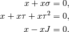
Finally,
![[P,g] + [P,g]J &=
g(P\{0,\infty\}) - gJ(J^{-1} P \{gJ(0), gJ(\infty)\}\\
&= (gP)\{g(0),g(\infty)\} - (gP) \{g(0),g(\infty)\}\\
&= 0,](_images/math/35f9388a5f953580a79ab21c15c2087a3fe1f8e2.png)
where we use that  acts trivially via linear fractional
transformations. This proves that the
listed relations are all satisfied.
acts trivially via linear fractional
transformations. This proves that the
listed relations are all satisfied.
That the listed relations are all relations is more difficult to
prove. One
approach is to show (as in [Mer94, Section 1.3]) that the quotient
of Manin symbols by the above relations and torsion is isomorphic to a
space of Shokurov symbols, which is in turn isomorphic to
. A much better approach is to apply some results
from group cohomology, as in
[Wie05].
If is a finite index subgroup and we have an algorithm to
enumerate the right cosets and to decide
which coset an arbitrary element of belongs to, then
Theorem 1.25 and the algorithms of Chapter Linear Algebra
yield an algorithm to compute  .
Note that if
.
Note that if  , then the relation
  is automatic.
Remark 1.26
The matrices  and
and  do not commute,
so in computing ,
one cannot first quotient out by the two-term
relations, then quotient out only the remaining free generators
by the relations, and get the right answer in general.
do not commute,
so in computing ,
one cannot first quotient out by the two-term
relations, then quotient out only the remaining free generators
by the relations, and get the right answer in general.
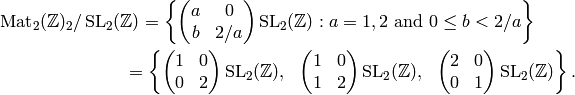
Coset Representatives and Manin Symbols
The following is analogous to Proposition 3.10:
Proposition 1.27
The right cosets  are in bijection
with pairs
are in bijection
with pairs  where
where  and
and  .
The coset containing
a matrix
.
The coset containing
a matrix  corresponds to .
Proof
This proof is copied from [Cre92, pg. 203],
except in that paper Cremona works with
the analogue of  in
in  , so
his result is slightly different.
Suppose
, so
his result is slightly different.
Suppose 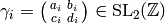 ,
for
,
for  .
We have
.
We have

which is in if and only if
(1)
and
(2)
Since the  have determinant
  , if
, if  ,
then the congruences (1)–(2) hold.
Conversely, if (1)–(2) hold, then
,
then the congruences (1)–(2) hold.
Conversely, if (1)–(2) hold, then
and likewise

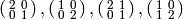
Thus we may view weight Manin symbols for as triples
of integers  , where
  and
and  with . Here corresponds to the Manin symbol
![[X^iY^{k-2-i}, \abcd{a}{b}{c'}{d'}]](_images/math/6b7205ff55457880f9cec011200c9955fcbc7f32.png) , where
, where  and
and  are
congruent to
are
congruent to  . The relations of
Theorem 1.25 become
. The relations of
Theorem 1.25 become
Recall that Proposition 3.10
gives a similar description for  .
.
Modular Symbols with Character
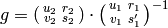
Suppose  Define an action of diamond-bracket operators
  o,
with
o,
with  on
Manin symbols as follows:
on
Manin symbols as follows:
![\langle d \rangle ([P,(u,v)]) = \left[P,(du, dv)\right].](_images/math/b5363f8809a513dc582704c89802f4a39b5c3e46.png)
Let
be a Dirichlet character, where  is
an
is
an  root of unity and is the order of
  .
Let
.
Let  be the quotient of
![\sM_k(\Gamma_1(N);\Z[\zeta])](_images/math/86b423cade7cce81c0d24ce0ef8c34314e6c4c48.png) by the relations (given
in terms of Manin symbols)
by the relations (given
in terms of Manin symbols)
for all ![x\in \sM_k(\Gamma_1(N);\Z[\zeta])](_images/math/80c820ee478e3ab97c1058691c231f083e2edc50.png) ,
,
 , and by any -torsion.
Thus is a
, and by any -torsion.
Thus is a ![\Z[\eps]](_images/math/0eea7aad9822a2bd7ceabad9ddf26ba553f62002.png) -module
that has no torsion when viewed as a -module.
-module
that has no torsion when viewed as a -module.
Hecke Operators
Suppose  is a subgroup of of level
  that contains .
Just as for modular forms, there is a commutative Hecke algebra
that contains .
Just as for modular forms, there is a commutative Hecke algebra
![\T=\Z[T_1,T_2, \ldots]](_images/math/a10276e35a525005fbee7d9ee05ae1c88c9d012a.png) , which is the subring of
, which is the subring of  generated by all Hecke operators.
Let
generated by all Hecke operators.
Let
where we omit  if
if  . Then
the Hecke operator
. Then
the Hecke operator  on
on  is given by
Notice when  that is defined by summing over
 matrices that correspond to the subgroups of
  of index
  . This is exactly how we defined on modular forms
in Definition Definition 2.26.
. This is exactly how we defined on modular forms
in Definition Definition 2.26.
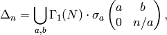
General Definition of Hecke Operators
Let be a finite index subgroup of and suppose

is a set such that  and
and  is finite. For example,
  satisfies this condition. Also,
if
satisfies this condition. Also,
if  , then for any positive integer , the set

also satisfies this condition, as we will now prove.
Lemma 1.28
We have

and
where 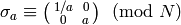 ,
the union is disjoint and
,
the union is disjoint and  with
with  ,
,  ,
and
,
and  . In particular, the set of cosets
 is finite.
Proof
(This is Lemma 1 of [Mer94, Section 2.3].)
If  and
and  , then

Thus 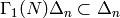 , and since
is a group,
, and since
is a group,  ; likewise
 .
.
For the coset decomposition, we first prove the statement for  , i.e., for
 . If
. If  is an arbitrary element
of
is an arbitrary element
of  with determinant , then using row operators on the left
with determinant , i.e., left multiplication by elements of ,
we can transform into the form
with determinant , then using row operators on the left
with determinant , i.e., left multiplication by elements of ,
we can transform into the form  , with
 and
and  . (Just imagine applying the Euclidean
algorithm to the two entries in the first column of . Then
. (Just imagine applying the Euclidean
algorithm to the two entries in the first column of . Then  is the
  of the two entries in the first column, and the lower left
entry is
of the two entries in the first column, and the lower left
entry is  . Next subtract
  from
from  until .)
Next suppose is arbitrary. Let  be such
that
be such
that

is a disjoint union. If  is arbitrary, then
as we showed above, there is some
is arbitrary, then
as we showed above, there is some  , so that
 , with and
, and . Write
, with and
, and . Write  , with
  .
Then
.
Then
It follows that
Since  and ,
there is
and ,
there is  such
that
such
that
We may then choose  .
Thus every
.
Thus every  is of the form
 ,
with and
,
with and  suitably bounded. This
proves the second claim.
suitably bounded. This
proves the second claim.
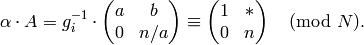
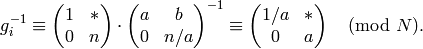
Let any element  act on the left on modular symbols
  by
by

(Until now we had only defined an action of
on modular symbols.)
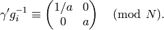
For  , let
, let
(3)
Note that  .
Also,
.
Also,  ,
where we set
,
where we set

Suppose and  are as above. Fix
a finite set of representatives for
are as above. Fix
a finite set of representatives for  .
Let
.
Let
be the linear map
This map is well defined because
if  and
and  ,
then
,
then
where we have used that  , and
acts trivially on
, and
acts trivially on  .
.
Let and  . Then the
Hecke operator
. Then the
Hecke operator  is
is  , and by Lemma 1.28,
where are as in Lemma 1.28.
Given this definition, we can compute the Hecke operators on
 as follows. Write as a modular symbol
, compute
as follows. Write as a modular symbol
, compute  as a modular symbol,
and then convert to Manin symbols using continued fractions
expansions. This is extremely inefficient; fortunately Lo”{i}c
Merel (following [Maz73]) found a much better way, which
we now describe (see [Mer94]).
as a modular symbol,
and then convert to Manin symbols using continued fractions
expansions. This is extremely inefficient; fortunately Lo”{i}c
Merel (following [Maz73]) found a much better way, which
we now describe (see [Mer94]).
Hecke Operators on Manin Symbols
If  is a subset of
  ,
let
,
let
where  is as in (3).
Also, for any ring and any subset
is as in (3).
Also, for any ring and any subset  ,
let
,
let ![R[S]](_images/math/de20eacb8a083748cf5fd4fd578dbd6079d1faed.png) denote the free -module with basis the elements of ,
so the elements of are the finite -linear combinations
of the elements of .
denote the free -module with basis the elements of ,
so the elements of are the finite -linear combinations
of the elements of .
One of the main theorems of [Mer94] is that for any
 satisfying the condition at the beginning of
Section General Definition of Hecke Operators, if we can find
satisfying the condition at the beginning of
Section General Definition of Hecke Operators, if we can find ![\sum u_M M \in
\C[\Mat_2(\Z)]](_images/math/25141c42b9205d46889606e52c969c97d9ce8af1.png) and a map
and a map
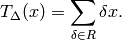
that satisfies certain conditions, then for any Manin
symbol ![[P,g] \in \M_k(\Gamma)](_images/math/bbc47b2db4d2eb2a5757d43e269619a3a9ef09c2.png) , we have
, we have
![T_\Delta([P,g]) =
\sum_{gM\in \tilde{\Delta}\SL_2(\Z)\text{ with }M\in\SL_2(\Z)} u_M
[\tilde{M}\cdot P,\,\, \phi(gM)].](_images/math/1f8cf19d57e827eec52c6b817157e458f3ad6ec6.png)
The paper
[Mer94] contains many examples of  and that satisfy all of the conditions.
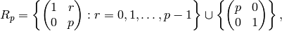
When , the complicated list of conditions becomes
simpler. Let  be the set of
  matrices with determinant .
An element
matrices with determinant .
An element
![h = \sum u_M [M] \in \C[\Mat_2(\Z)_n]](_images/math/b994a0129c22881338daa6eb10a2cdeebc774e28.png)
satisfies condition  if for every
  , we have that
(4)![\sum_{M \in K} u_M([M\infty] - [M 0 ]) = [\infty] - [0]
\in \C[P^1(\Q)].](_images/math/a6173339113c58a10fabb23cce6433c344396a34.png)
If  satisfies condition , then for any Manin symbol
![[P,g] \in M_k(\Gamma_1(N))](_images/math/2c5fc45e9d696ea113824e44e499729de1f7393e.png) , Merel proves that
, Merel proves that
(5)![T_n([P,(u,v)]) = \sum_{M} u_M [P(aX+bY, \, cX+dY), (u,v)M].](_images/math/c5771b3cefd87429dafe6bdbe0646d9b4ab80a3b.png)
Here  corresponds via Proposition 1.27
to a coset of in , and
if
corresponds via Proposition 1.27
to a coset of in , and
if  and
and 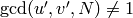 ,
then we omit the corresponding summand.
,
then we omit the corresponding summand.
For example, we will now check directly that the element
![h_2 = \left[\mtwo{2}{0}{0}{1}\right] +
\left[\mtwo{1}{0}{0}{2}\right] +
\left[\mtwo{2}{1}{0}{1}\right] +
\left[\mtwo{1}{0}{1}{2}\right]](_images/math/7009d290f8b9589319ec50f095491bfa0eb9798e.png)
satisfies condition  .
We have, as in the proof of Lemma 1.28
(but using elementary column operations), that
.
We have, as in the proof of Lemma 1.28
(but using elementary column operations), that
To verify condition , we consider in turn each of the three
elements of  and check that (4)
holds. We have that
and check that (4)
holds. We have that
and
Thus if  , the left
sum of (4) is
, the left
sum of (4) is
![[\abcd{1}{0}{0}{2}(\infty)] - [\abcd{1}{0}{0}{2}(0)] = [\infty]-[0]](_images/math/33bf2e6f6cd021e4134a4630782e88e35cbbc160.png) ,
as required. If
,
as required. If  , then
the left side of (4) is
, then
the left side of (4) is
![[\abcd{2}{1}{0}{1}(\infty)] &- [\abcd{2}{1}{0}{1}(0)]
+ [\abcd{1}{0}{1}{2}(\infty)] - [\abcd{1}{0}{1}{2}(0)] \\
&= [\infty] - [1] + [1] - [0] = [\infty] - [0].](_images/math/45cfc80497c7c4e6f1ec57c199a5d67d2402b904.png)
Finally, for  we also have
![[\abcd{2}{0}{0}{1}(\infty)] - [\abcd{2}{0}{0}{1}(0)] = [\infty]-[0]](_images/math/1d8be5ae4c73aa3b071b79c8b825012a68c4f2d4.png) ,
as required.
Thus by (5) we can compute
,
as required.
Thus by (5) we can compute  on any Manin
symbol, by summing over the action
of the four matrices
on any Manin
symbol, by summing over the action
of the four matrices
 .
.
Proposition 1.29
The element
![\sum_{\substack{a>b\geq 0\\d>c\geq 0\\ad-bc=n}}
\left[\mtwo{a}{b}{c}{d}\right] \in \Z[\Mat_2(\Z)_n]](_images/math/3472e0c1346ecd84617df08dcddf0d9139d2f038.png)
satisfies condition .
Merel’s two-page proof of Proposition 1.29 is fairly elementary.
Remark 1.30
In [Cre97a, Section 2.4], Cremona discusses the work of Merel
and Mazur on Heilbronn matrices in the special cases
 and weight
  . He gives a simple proof
that the action of on Manin symbols can be computed by summing
the action of some set
. He gives a simple proof
that the action of on Manin symbols can be computed by summing
the action of some set  of matrices of determinant . He
then describes the set and gives an efficient continued
fractions algorithm for computing it (but he does not prove
that his satisfy Merel’s hypothesis).
of matrices of determinant . He
then describes the set and gives an efficient continued
fractions algorithm for computing it (but he does not prove
that his satisfy Merel’s hypothesis).
Remarks on Complexity
Merel gives another family  of matrices
that satisfy condition , and he proves that
as
of matrices
that satisfy condition , and he proves that
as  ,
,
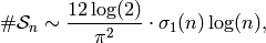
where  is the sum of the divisors of .
Thus for a fixed space of modular symbols,
one can compute using
is the sum of the divisors of .
Thus for a fixed space of modular symbols,
one can compute using
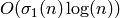 arithmetic operations.
Note that we have fixed , so we ignore
the linear algebra involved in computation of a presentation; also, adding
elements takes a bounded number of field operations when the space
is fixed. Thus, using Manin symbols
the complexity of computing , for prime, is
arithmetic operations.
Note that we have fixed , so we ignore
the linear algebra involved in computation of a presentation; also, adding
elements takes a bounded number of field operations when the space
is fixed. Thus, using Manin symbols
the complexity of computing , for prime, is 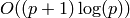 field operations, which is exponential in the number of digits
of .
field operations, which is exponential in the number of digits
of .
Basmaji’s Trick
There is a trick of Basmaji (see [Bas96]) for computing
a matrix of on , when is very large, and it is more
efficient than one might naively expect. Basmaji’s trick does not
improve the big-oh complexity for a fixed space, but it
does improve the
complexity by a constant factor of the dimension of  .
Suppose we are interested in computing the matrix for for some massive
integer and that has large dimension.
The trick is as follows. Choose a list
.
Suppose we are interested in computing the matrix for for some massive
integer and that has large dimension.
The trick is as follows. Choose a list
![x_1 =[P_1,g_1],\ldots,x_r = [P_r,g_r] \in V = \sM_k(\Gamma;\Q)](_images/math/61f5419ee928e6c9c6b67edd841c9543169d13fc.png)
of Manin symbols such that the map  given by
is injective. In practice, it is often possible to do this with  “very small”.
Also, we emphasize that
“very small”.
Also, we emphasize that  is a
is a  -vector space of dimension
 .
.
Next find Hecke operators  , with
  small,
whose images form a basis for the image of
small,
whose images form a basis for the image of  .
Now with the above data precomputed, which only required working with
Hecke operators for small , we are ready to compute
with huge. Compute
.
Now with the above data precomputed, which only required working with
Hecke operators for small , we are ready to compute
with huge. Compute  , for each
  ,
which we can compute using Heilbronn matrices since each
,
which we can compute using Heilbronn matrices since each
![x_i=[P_i,g_i]](_images/math/dd0eca2526d8754efbda36f4cb40e155a9a7a5c5.png) is a Manin symbol. We thus obtain
is a Manin symbol. We thus obtain  Since we have precomputed Hecke operators
  such that
 generate , we can find
  such that
 . Then since
is injective, we have
. Then since
is injective, we have  , which gives
the full matrix of on
, which gives
the full matrix of on  .
.
Cuspidal Modular Symbols
Let  be the free abelian group on symbols
  ,
for
,
for  , and set
![\sB_k = \Z[X,Y]_{k-2}\tensor\sB.](_images/math/ddca2f3bf432936e42f9e44a6f31a65701cb4561.png)
Define a left action of on  by
by
for .
For any finite index subgroup  ,
let
,
let
 be the quotient of by the relations
 for all
  and by any torsion. Thus
is a torsion-free abelian group.
and by any torsion. Thus
is a torsion-free abelian group.
The boundary map is the map
given by extending the map

linearly.
The space  of cuspidal modular symbols
is the kernel
of cuspidal modular symbols
is the kernel

so we have an exact sequence

One can prove that when  ,
this sequence is exact on the right.
,
this sequence is exact on the right.
Next we give a presentation of in terms of
“boundary Manin symbols”.
Boundary Manin Symbols
We give an explicit description of the boundary
map in terms of Manin symbols for
, then describe an
efficient way to compute the boundary map.
Let  be the equivalence relation
on
be the equivalence relation
on  given by
![[\Gamma\smallvtwo{\lambda u}{\lambda v}] \sim
\sign(\lambda)^k[\Gamma\smallvtwo{u}{v}],](_images/math/fcacefbd41a72692db1b7c6361accb82c698c1a6.png)
for any  . Denote by
  the finite-dimensional -vector space
with basis the equivalence classes
the finite-dimensional -vector space
with basis the equivalence classes
 .
The following two propositions are proved in [Mer94].
.
The following two propositions are proved in [Mer94].
Proposition 1.31
The map
![\mu:\sB_k(\Gamma)\ra B_k(\Gamma),
\qquad P\left\{\frac{u}{v}\right\}\mapsto
P(u,v)\left[\Gamma\vtwo{u}{v}\right]](_images/math/9559cf5b615be0e86100a208d28fa2fffe8586f1.png)
is well defined and injective.
Here  and
and  are assumed coprime.
Thus the kernel of  is the same as the kernel of
  .
.
Proposition 1.32
Let  and
and  . We have
![\mu\circ\delta([P,(c,d)])
= P(1,0)[\Gamma\smallvtwo{a}{c}]
-P(0,1)[\Gamma\smallvtwo{b}{d}].](_images/math/d18d366f2bb5581342c7baa2bbd9ffa0439431af.png)
We next describe how to explicitly compute
 by generalizing the algorithm of [Cre97a, Section 2.2].
To compute the image of
by generalizing the algorithm of [Cre97a, Section 2.2].
To compute the image of ![[P,(c,d)]](_images/math/7ee56748b3815f654fd127c6f4fb0420331cfed4.png) , with
,
we must compute the class of
, with
,
we must compute the class of ![[\smallvtwo{a}{c}]](_images/math/12560333bc7439a91fe0623e008f6836b93e3f84.png) and of
and of
![[\smallvtwo{b}{d}]](_images/math/26869b643da3caa086a9fad68012b97aafc6ba9f.png) .
Instead of finding a canonical form for cusps, we
use a quick test for equivalence modulo scalars.
In the following algorithm, by the
.
Instead of finding a canonical form for cusps, we
use a quick test for equivalence modulo scalars.
In the following algorithm, by the  symbol we mean
the basis vector for a basis of
symbol we mean
the basis vector for a basis of  . This
basis is constructed as the algorithm is called successively.
We first give the algorithm, and then prove the facts
used by the algorithm in testing equivalence.
. This
basis is constructed as the algorithm is called successively.
We first give the algorithm, and then prove the facts
used by the algorithm in testing equivalence.
Algorithm 1.33
Given a boundary Manin symbol ![[\smallvtwo{u}{v}],](_images/math/694f8e5701fe7de3d787b83d633af21910bd14b0.png) this algorithm outputs an integer and a
scalar
this algorithm outputs an integer and a
scalar  such that
 ![[\smallvtwo{u}{v}]](_images/math/493bbe978d5477aa4f8cede37b08d420eff2ba7d.png) is equivalent to
times the symbol found so far. (We call this algorithm
repeatedly and maintain a running list of cusps seen so far.)
is equivalent to
times the symbol found so far. (We call this algorithm
repeatedly and maintain a running list of cusps seen so far.)
- Use Proposition 3.21 to check
whether or not is equivalent, modulo scalars, to
any cusp found. If so, return the representative, its
index, and the scalar. If not, record
 in the
representative list.
in the
representative list. - Using Proposition 1.37,
check whether or not is forced to equal by the
relations. If it does not equal , return its position in the list
and the scalar . If it equals , return the scalar and the
position ; keep in the list, and record that it
is equivalent to .
The case considered in Cremona’s book [Cre97a] only involve the trivial character, so no cusp classes are forced to vanish. Cremona gives the following two criteria for equivalence.
Proposition 1.34
Consider  , , with
  integers such
that
integers such
that  for each .
There exists
 such that
 if and only if
There exists
 such that
if and only if
such that
if and only if
Algorithm 1.35
Suppose  and
and
 are equivalent modulo .
This algorithm computes a matrix such
that .
are equivalent modulo .
This algorithm computes a matrix such
that .
- Let
 be solutions to
 and
and
 .
. - Find integers
 and
and  such
that
such
that  .
. - Let
 and
and  .
. - Output
 ,
which sends to .
,
which sends to .
Proof
See the proof of [Cre97a, Prop. 8.13].
The relations can make the situation more
complicated, since it is possible that
 but
but
![\eps(\alp)\left[\vtwo{u}{v}\right] =\left[\gamma_\alp \vtwo{u}{v}\right]=
\left[\gamma_\beta \vtwo{u}{v}\right]=\eps(\beta)\left[\vtwo{u}{v}\right].](_images/math/36b0cc57157698a76d6984c4df7cc86e74ee0217.png)
One way out of this difficulty is to construct
the cusp classes for , and then quotient
out by the additional relations using
Gaussian elimination. This is far too
inefficient to be useful in practice because the number of
cusp classes can be unreasonably large.
Instead, we give a quick test to determine whether or not
a cusp vanishes modulo the -relations.
Lemma 1.36
Suppose and  are integers
such that
are integers
such that  .
Then there exist integers
.
Then there exist integers  and
and  ,
congruent to and modulo , respectively,
such that
,
congruent to and modulo , respectively,
such that  .
.
Proof
By Exercise 1.12 the map
 is surjective.
By the Euclidean algorithm, there exist
integers ,
is surjective.
By the Euclidean algorithm, there exist
integers ,  and
and  such that
 .
Consider the matrix
.
Consider the matrix
 and take , to be the bottom
row of a lift of this matrix to .
and take , to be the bottom
row of a lift of this matrix to .
Proposition 1.37
Let be a positive integer and a Dirichlet
character of modulus .
Suppose is a cusp with and coprime.
Then vanishes modulo the relations
![\left[\gamma\smallvtwo{u}{v}\right]=
\eps(\gamma)\left[\smallvtwo{u}{v}\right],\qquad
\text{all $\gamma\in\Gamma_0(N)$},](_images/math/c9edd7837260f937bc532809ea7032fa9c7bd104.png)
if and only if there exists  ,
with
,
with  , such that
Proof
First suppose such an exists.
By Lemma 1.36
there exists  lifting
 such that .
The cusp
such that .
The cusp  has coprime coordinates so,
by Proposition 1.34 and our
congruence conditions on , the cusps
has coprime coordinates so,
by Proposition 1.34 and our
congruence conditions on , the cusps
 and are equivalent by
an element of .
This implies that
and are equivalent by
an element of .
This implies that ![\left[\smallvtwo{\beta{}u}{\beta'{}v}\right]
=\left[\smallvtwo{u}{v}\right]](_images/math/cd67f0f112bd578d2c3ee985203c072e087f4c9f.png) .
Since
.
Since ![\left[\smallvtwo{\beta{}u}{\beta'{}v}\right]
= \eps(\alp)\left[\smallvtwo{u}{v}\right]](_images/math/47ee1721d0c8c1083e2967dcfa0582d8d2899bc7.png) and , we have
and , we have ![\left[\smallvtwo{u}{v}\right]=0](_images/math/b039b2c8608916f5b455971844e755c53ce7bfe7.png) .
.
Conversely, suppose .
Because all relations are two-term relations and the
-relations identify -orbits,
there must exists and with
![\left[\gamma_\alp \vtwo{u}{v}\right]
=\left[\gamma_\beta \vtwo{u}{v}\right]
\qquad\text{ and }\eps(\alp)\ne \eps(\beta).](_images/math/3876ea7329cbbcd61acf5af05d487075376c5030.png)
Indeed, if this did not occur,
then we could mod out by the relations by writing
each ![\left[\gamma_\alp \smallvtwo{u}{v} \right]](_images/math/805f1c5ca7264745717f41d590f554baa4a4a397.png) in terms of
in terms of ![\left[\smallvtwo{u}{v}\right]](_images/math/00e466ff071d039b32e3cf1b80d2546c398caa85.png) , and there would
be no further relations left to kill
.
Next observe that
, and there would
be no further relations left to kill
.
Next observe that
![\left[\gamma_{\beta^{-1}\alp}
\vtwo{u}{v}\right]
&= \left[\gamma_{\beta^{-1}}\gamma_\alp
\vtwo{u}{v}\right]\\
&= \eps(\beta^{-1})\left[\gamma_\alp
\vtwo{u}{v}\right]
= \eps(\beta^{-1})\left[\gamma_\beta
\vtwo{u}{v}\right]
= \left[\vtwo{u}{v}\right].](_images/math/cd694666885caf7a9f1f3e981b4ac41f8b7b032a.png)
Applying Proposition 1.34 and
noting that  shows
that
shows
that  satisfies the properties
of the ” ” in the statement of the
proposition.
satisfies the properties
of the ” ” in the statement of the
proposition.
We enumerate the possible appearing
in Proposition 1.37 as follows.
Let  and list the
 , for
, for  ,
such that
,
such that  .
.
Pairing Modular Symbols and Modular Forms
In this section we define a pairing between modular symbols and modular forms that the Hecke operators respect. We also define an involution on modular symbols and study its relationship with the pairing. This pairing is crucial in much that follows, because it gives rise to period maps from modular symbols to certain complex vector spaces.
Fix an integer weight and a finite index subgroup
of . Let  denote the space
of holomorphic modular forms of weight for ,
and let
denote the space
of holomorphic modular forms of weight for ,
and let  denote its cuspidal subspace.
Following [Mer94, Section 1.5], let
denote its cuspidal subspace.
Following [Mer94, Section 1.5], let
(6)
denote the space of antiholomorphic cusp forms. Here
 is the function on
  given by
 .
.
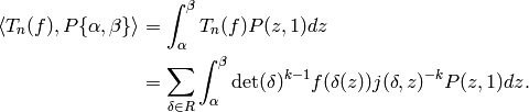
Define a pairing
(7)
by letting

and extending linearly. Here the integral is a complex
path integral along a simple path from  to in
to in  (so, e.g., write
  ,
where
,
where  traces out the path and consider
two real integrals).
traces out the path and consider
two real integrals).
Proposition 1.38
The integration pairing is well defined, i.e., if we
replace by an equivalent modular symbol
(equivalent modulo the left action of ), then the integral
is the same.
Proof
This follows from the change of variables formulas
for integration and the fact that  and
and
 . For example, if
  ,
and
,
and  , then
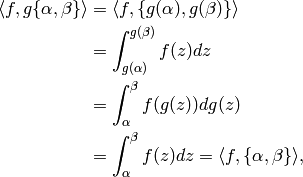
where 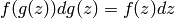 because
 is a weight modular form.
For the case of arbitrary weight , see
Exercise 1.14.
is a weight modular form.
For the case of arbitrary weight , see
Exercise 1.14.
The integration pairing is very relevant to the
study of special values of
 -functions. The -function
of a cusp form
-functions. The -function
of a cusp form 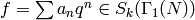 is
is
(8)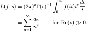
The equality of the integral and the
Dirichlet series follows
by switching the order of summation and integration,
which is justified using standard estimates on  (see, e.g., [Kna92, Section VIII.5]).
For each integer  with
with  , we have,
setting
, we have,
setting  and making the change of variables
  in (8), that
(9)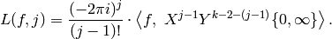
The integers as above are called critical integers.
When is an eigenform, they have deep
conjectural significance (see [BK90, Sch90]).
One can approximate  to any desired precision
by computing the above pairing explicitly using
the method described in Chapter Computing Periods.
Alternatively, [Dok04] contains
methods for computing special values of very
general -functions, which can be used for
approximating
to any desired precision
by computing the above pairing explicitly using
the method described in Chapter Computing Periods.
Alternatively, [Dok04] contains
methods for computing special values of very
general -functions, which can be used for
approximating  for arbitrary
  , in addition
to just the critical integers
, in addition
to just the critical integers  .
.
Theorem 1.39
The pairing

is a nondegenerate pairing of complex vector spaces.
Corollary 1.40
We have

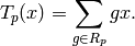
The pairing is also compatible with Hecke operators. Before proving
this, we define an action of Hecke operators on and
on  . The definition is similar to the one
we gave in Section Hecke Operators for modular forms of level .
For a positive integer , let
. The definition is similar to the one
we gave in Section Hecke Operators for modular forms of level .
For a positive integer , let  be a set of coset
representatives for from
Lemma 1.28. For any
be a set of coset
representatives for from
Lemma 1.28. For any  and
and  set
set
![f^{[\gamma]_k} = \det(\gamma)^{k-1} (cz+d)^{-k} f(\gamma(z)).](_images/math/bff7a83af850b2fdab4cb1b4e8046e96f6f77d5d.png)
Also, for  , set
, set
![f^{[\gamma]_k'} = \det(\gamma)^{k-1} (c\zbar+d)^{-k} f(\gamma(z)).](_images/math/48de977b97539384d3146dcc82bbf62a2ffc6aaf.png)
Then for ,
![T_n(f) = \sum_{\gamma\in R_n} f^{[\gamma]_k}](_images/math/107c047c94d6c915422bf209aa4a1868afa9fb41.png)
and for ,
![T_n(f) = \sum_{\gamma\in R_n} f^{[\gamma]_k'}.](_images/math/8f2c5ba1e839ace16f527fb48cee5ffcd14ae2fb.png)
This agrees with the definition from Section Hecke Operators
when .
Remark 1.41
If is an arbitrary finite index subgroup of ,
then we can define operators  on
for any with
on
for any with  and finite. For concreteness we
do not do the general case here or in the theorem below, but
the proof is exactly the same (see [Mer94, Section 1.5]).
and finite. For concreteness we
do not do the general case here or in the theorem below, but
the proof is exactly the same (see [Mer94, Section 1.5]).
Finally we prove the promised Hecke compatibility of the pairing. This proof should convince you that the definition of modular symbols is sensible, in that they are natural objects to integrate against modular forms.
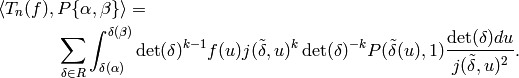
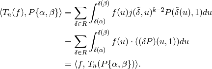
Theorem 1.42
If

and  , then for any ,
Proof
We follow [Mer94, Section 2.1] (but with more details) and will
only prove the theorem when  , the proof
in the general case being the same.
, the proof
in the general case being the same.
Let  , ,
and for
, ,
and for  , set
, set
Let be any positive integer,
and let be a set of coset
representatives for from
Lemma 1.28.
We have
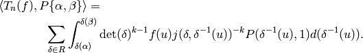
Now for each summand corresponding to the  ,
make the change of variables
,
make the change of variables  . Thus we
make
. Thus we
make  change of variables.
Also, we will use the notation
change of variables.
Also, we will use the notation
for  .
We have
.
We have
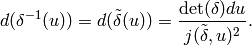
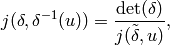
We have  ,
since a linear fractional transformation is unchanged
by a nonzero rescaling of a matrix that induces it.
Thus by the quotient rule, using that
,
since a linear fractional transformation is unchanged
by a nonzero rescaling of a matrix that induces it.
Thus by the quotient rule, using that  has determinant
  , we see that
We next show that
(10)
From the definitions, and again using that 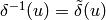 , we see that
which proves that (10) holds. Thus
Next we use that

To see this, note that  .
Using this we see that
.
Using this we see that
Now substituting  for
for  , we see that

as required. Thus finally
Suppose that is a finite index
subgroup of such that
if  , then

For example, satisfies this condition.
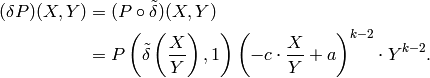
There is an involution  on given by
(11)
which we call the star involution.
On Manin symbols, is
(12)![\iota^*[P,(u,v)] = -[P(-X,Y), (-u,v)].](_images/math/bf0bd00c3d527d0e21eb74748e3b1bf7913af18a.png)
Let  be the
  eigenspace for
on , and let
eigenspace for
on , and let  be the
  eigenspace.
There is also a map
eigenspace.
There is also a map  on modular forms, which
is adjoint to .
on modular forms, which
is adjoint to .
Remark 1.43
Notice the minus sign in front of  in
(11). This sign is missing in [Cre97a],
which is a potential source of confusion (this is not a mistake,
but a different choice of convention).
in
(11). This sign is missing in [Cre97a],
which is a potential source of confusion (this is not a mistake,
but a different choice of convention).
We now state the final result about the pairing, which explains how modular symbols and modular forms are related.
Theorem 1.44
The integration pairing  induces
nondegenerate Hecke compatible bilinear pairings
induces
nondegenerate Hecke compatible bilinear pairings

Remark 1.45
We make some remarks about computing
the boundary map of Section Boundary Manin Symbols when working
in the  quotient.
Let be a sign, either
or . To compute
quotient.
Let be a sign, either
or . To compute  , it is necessary to replace
by its quotient modulo the additional relations
, it is necessary to replace
by its quotient modulo the additional relations ![\left[
\smallvtwo{-u}{\hfill v}\right] = s \left[\smallvtwo{u}{v}\right]](_images/math/d81c3ef673b68efeca983038c1b41517fb841327.png) for all cusps . Algorithm 1.33 can be
modified to deal with this situation as follows. Given a cusp
for all cusps . Algorithm 1.33 can be
modified to deal with this situation as follows. Given a cusp
 , proceed as in Algorithm 1.33 and
check if either or
, proceed as in Algorithm 1.33 and
check if either or  is
equivalent (modulo scalars) to any cusp seen so far. If not, use the
following trick to determine whether the and -relations kill
the class of : use the unmodified
Algorithm 1.33 to compute the scalars
is
equivalent (modulo scalars) to any cusp seen so far. If not, use the
following trick to determine whether the and -relations kill
the class of : use the unmodified
Algorithm 1.33 to compute the scalars  and indices
  ,
,  associated to and
, respectively. The -relation kills the
class of if and only if
associated to and
, respectively. The -relation kills the
class of if and only if  but
but  .
.
Degeneracy Maps
In this section, we describe natural maps between spaces of modular symbols with character of different levels. We consider spaces with character, since they are so important in applications.
Fix a positive integer and a Dirichlet
character
 . Let
. Let  be a positive divisor
of that is divisible by the conductor of , in the sense
that factors through
be a positive divisor
of that is divisible by the conductor of , in the sense
that factors through  via the natural map
 composed with some uniquely defined
character
composed with some uniquely defined
character  . For any positive divisor
  of
of
 , let
, let  and fix a choice
  of coset representatives for
  .
.
Remark 1.46
Note that [Mer94, Section 2.6] contains a typo:
The quotient ”  ” should be replaced
by ”
” should be replaced
by ”  “.
“.
Proposition 1.47
For each divisor of there are well-defined linear maps
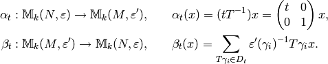
Furthermore,
 is multiplication by
![t^{k-2}\cdot [\Gamma_0(M) : \Gamma_0(N)].](_images/math/3d7cfe7d71374bdc3a5a5410c79a119d672b63f0.png)
Proof
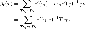
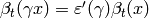
To show that  is well defined, we must show that for
each
is well defined, we must show that for
each  and
and  ,
we have
,
we have

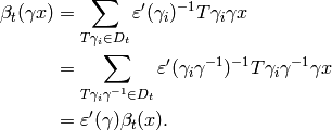
We have

so

We next verify that  is well defined.
Suppose that
is well defined.
Suppose that  and
and  ;
then
;
then 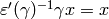 , so
, so
This computation shows that the definition of
does not depend on the choice  of coset representatives.
To finish the proof that is well defined,
we must show that, for , we have
of coset representatives.
To finish the proof that is well defined,
we must show that, for , we have
 so that
respects the relations that define
so that
respects the relations that define  .
Using that does not depend on the choice of
coset representative, we find that for ,
.
Using that does not depend on the choice of
coset representative, we find that for ,
To compute  , we use
that
, we use
that ![\#D_t = [\Gamma_0(N) : \Gamma_0(M)]](_images/math/a1f72960e556153105329f88cdbe912fa45a1ea7.png) :
:
![\alp_t(\beta_t(x)) &=
\alp_t \left(\sum_{T\gamma_i}
\eps'(\gamma_i)^{-1}T\gamma_i x\right)\\
&= \sum_{T\gamma_i}
\eps'(\gamma_i)^{-1}(tT^{-1})T\gamma_i x\\
&= t^{k-2}\sum_{T\gamma_i}
\eps'(\gamma_i)^{-1}\gamma_i x\\
&= t^{k-2}\sum_{T\gamma_i} x \\
&= t^{k-2} \cdot [\Gamma_0(N) : \Gamma_0(M)] \cdot x.](_images/math/d0bfeb913223cf3cd16e11dee6a2fe5862102c64.png)
The scalar factor of  appears instead
of , because is acting on as an element of
and not as an an element of .
appears instead
of , because is acting on as an element of
and not as an an element of .
Definition 1.48
The space  of new modular symbols is the
intersection of the kernels of the as
runs through all positive divisors of and
runs through positive divisors of strictly less than
and divisible by the conductor of .
The subspace
of new modular symbols is the
intersection of the kernels of the as
runs through all positive divisors of and
runs through positive divisors of strictly less than
and divisible by the conductor of .
The subspace  of old modular symbols
is the subspace generated by the images of the
where runs through all positive divisors of and
runs through positive divisors of strictly less than
and divisible by the conductor of .
The new and old subspaces of cuspidal modular
symbols are the intersections of the above spaces
with
of old modular symbols
is the subspace generated by the images of the
where runs through all positive divisors of and
runs through positive divisors of strictly less than
and divisible by the conductor of .
The new and old subspaces of cuspidal modular
symbols are the intersections of the above spaces
with  .
.
Example 1.49
The new and old subspaces need not be disjoint, as the following
example illustrates! (This contradicts [Mer94, pg. 80].)
Consider, for example, the case  , , and trivial character.
The spaces
, , and trivial character.
The spaces  and
and  are each of
dimension , and each is generated by the modular symbol
are each of
dimension , and each is generated by the modular symbol
 . The space
  is of dimension
  and is generated by the three modular symbols
  ,
,
 , and
, and  . The space generated by the two
images of under the two degeneracy maps has
dimension , and likewise for . Together
these images generate , so
is equal to its old subspace. However, the new subspace is
nontrivial because the two degeneracy maps
. The space generated by the two
images of under the two degeneracy maps has
dimension , and likewise for . Together
these images generate , so
is equal to its old subspace. However, the new subspace is
nontrivial because the two degeneracy maps  are equal, as are the two degeneracy maps

In particular, the
intersection of the kernels of the degeneracy maps has dimension at
least (in fact, it equals ).
We verify some of the above claims using Sage.
sage: M = ModularSymbols(Gamma0(6)); M
Modular Symbols space of dimension 3 for Gamma_0(6)
of weight 2 with sign 0 over Rational Field
sage: M.new_subspace()
Modular Symbols subspace of dimension 1 of Modular
Symbols space of dimension 3 for Gamma_0(6) of weight
2 with sign 0 over Rational Field
sage: M.old_subspace()
Modular Symbols subspace of dimension 3 of Modular
Symbols space of dimension 3 for Gamma_0(6) of weight
2 with sign 0 over Rational Field
Explicitly Computing  
In this section we explicitly compute for various
and . We represent Manin symbols for as triples
of integers  , where
  , and corresponds
to
, and corresponds
to ![[X^i Y^{k-2-i}, (u,v)]](_images/math/6d24bb9e2eff0259b7df365055c0ee30730f1ba7.png) in the usual notation. Also, recall from
Proposition 3.10 that
in the usual notation. Also, recall from
Proposition 3.10 that  corresponds to the right
coset of that contains a matrix
with
corresponds to the right
coset of that contains a matrix
with  as elements of
 , i.e., up to rescaling by an element of
  .
.
Computing 
In this section we give an algorithm to compute a canonical
representative for each element of . This algorithm is
extremely important because modular symbols implementations use it a
huge number of times. A more naive approach would be to store all
pairs and a fixed reduced representative, but
this wastes a huge amount of memory. For example, if  ,
we would store an array of
,
we would store an array of

Another approach to enumerating is described at the end
of [Cre97a, Section 2.2]. It uses the fact that is easy to
test whether two pairs  define the same element
of ; they do if and only if we have equality of cross
terms
define the same element
of ; they do if and only if we have equality of cross
terms  (see
[Cre97a, Prop. 2.2.1]). So we consider the
-based list of elements
(see
[Cre97a, Prop. 2.2.1]). So we consider the
-based list of elements
(13)
concatenated with the list of nonequivalent elements
 for
for  and
and
 , checking each time we add a new element to our
list (of ) whether we have already seen it.
, checking each time we add a new element to our
list (of ) whether we have already seen it.
Given a random pair , the problem
is then to find the index of the element of our list of the equivalent
representative in .
We use the following
algorithm, which finds a canonical representative for each element of
. Given an arbitrary
, we first find the canonical equivalent elements  .
If
.
If  , then the index is
  . If
. If
 , we find the corresponding element
in an explicit sorted list, e.g., using binary search.
, we find the corresponding element
in an explicit sorted list, e.g., using binary search.
In the following algorithm,  denotes the residue of
modulo that satisfies
denotes the residue of
modulo that satisfies  .
Note that we never create and store the
list (13) itself in memory.
.
Note that we never create and store the
list (13) itself in memory.
Algorithm 1.50
Given and and a positive integer ,
this algorithm outputs
a pair  such that
  as
elements of and
as
elements of and  such that
  .
Moreover, the element
.
Moreover, the element  does not
depend on the class of , i.e., for any with
does not
depend on the class of , i.e., for any with  the input
  also outputs .
If is not in , this algorithm
outputs
also outputs .
If is not in , this algorithm
outputs  .
.
- [Reduce] Reduce both and modulo .
- [Easy
 Case] If
  , check that
  .
If so, return
.
If so, return  and ; otherwise return .
 - [GCD] Compute
 and
and  such that
  .
. - [Not in
 ?] We have
  , so if
 , then
  ,
and we return .
,
and we return . - [Pseudo-Inverse]
Now
 , so we may think of as “pseudo-inverse”
of
, so we may think of as “pseudo-inverse”
of  , in the sense that
  is as close as possible to
being modulo . Note that since
is as close as possible to
being modulo . Note that since  , changing modulo
 does not change
  . We can adjust modulo
so it is coprime to (by adding multiples of
to ). (This is because
. We can adjust modulo
so it is coprime to (by adding multiples of
to ). (This is because  , so
is a unit mod , and the map
, so
is a unit mod , and the map  is surjective, e.g., as we saw in the proof of
Algorithm 4.28.)
is surjective, e.g., as we saw in the proof of
Algorithm 4.28.) - [Multiply by ] Multiply by , and replace
by the
equivalent element
 of .
of . - [Normalize]
Compute the unique pair
 equivalent to
  that
minimizes , as follows:
that
minimizes , as follows:- [Easy Case] If
 , this pair is
  .
. - [Enumerate and Find Best]
Otherwise, note that if
 and
and
 , then
  , so
, so  for some with
  . Then for
  coprime to ,
we have
coprime to ,
we have  . So we compute
all pairs
. So we compute
all pairs  and pick out the one that minimizes the
least nonnegative residue of
and pick out the one that minimizes the
least nonnegative residue of  modulo .
 - [Invert and Output]
The that we computed in the above steps multiplies
the input to give the output . Thus we
invert it, since the scalar we output
multiplies to give .
- [Easy Case] If
Remark 1.51
In the above algorithm, there are many gcd’s with so one should
create a table of the gcd’s of  with .
Remark 1.52
Another approach is to instead use that
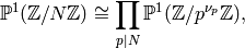
where  ,
and that it is relatively easy to enumerate the
elements of
,
and that it is relatively easy to enumerate the
elements of  for a prime power
  .
.
Algorithm 1.53
Given an integer  , this algorithm makes a sorted list of the
distinct representatives of with
, this algorithm makes a sorted list of the
distinct representatives of with
 , as output by Algorithm 1.50.
- For each
 with
with  do the
following:
do the
following:- Use Algorithm 1.50 to compute
the canonical representative equivalent to
 ,
and include it in the list.
,
and include it in the list. - If
 , for each
  with
with  and
and  , append the normalized representative
of to the list.
, append the normalized representative
of to the list.
- Use Algorithm 1.50 to compute
the canonical representative
- Sort the list.
- Pass through the sorted list and delete any duplicates.
Explicit Examples
Explicit detailed examples are crucial when implementing modular symbols algorithms from scratch. This section contains a number of such examples.
Examples of Computation of 
In this section, we compute explicitly in a few cases.
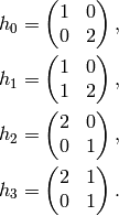
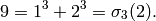
Example 1.54
We compute  . Because
  and
and 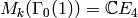 , we expect
  to have dimension
and for each integer the Hecke operator to have eigenvalue the
sum
to have dimension
and for each integer the Hecke operator to have eigenvalue the
sum  of the cubes of positive divisors of .
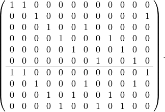
The Manin symbols are

The relation matrix is
where the first two rows correspond to -relations and the second
three to  -relations.
Note that we do not include all -relations, since it is obvious
that some are redundant, e.g.,
-relations.
Note that we do not include all -relations, since it is obvious
that some are redundant, e.g.,  and
and  are the same since has order .
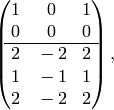
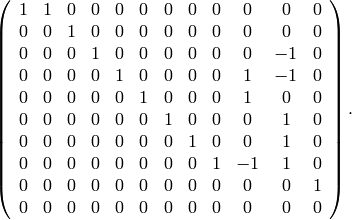
The echelon form of the relation matrix is

where we have deleted the zero rows from the bottom. Thus we may replace the above complicated list of relations with the following simpler list of relations:

from which we immediately read off that the second generator  is
and
is
and  . Thus
  has dimension , with
basis the equivalence class of
has dimension , with
basis the equivalence class of  (or of ).
Next we compute the Hecke operator on .
The Heilbronn matrices
of determinant from Proposition 1.29
are
To compute , we apply each of these matrices to ,
then reduce modulo the relations.
We have
![x_2\mtwo{1}{0}{0}{2} &= [X^2,(0,0)] \mtwo{1}{0}{0}{2}
x_2,\\
x_2 \mtwo{1}{0}{1}{2} &= [X^2,(0,0)] = x_2,\\
x_2 \mtwo{2}{0}{0}{1} &= [(2X)^2,(0,0)] = 4x_2,\\
x_2 \mtwo{2}{1}{0}{1} &= [(2X+1)^2,(0,0)] = x_0 + 4x_1 + 4x_2
\sim 3x_2.](_images/math/85819d95e89c3c4432b878e054e14036ee482fcd.png)
Summing we see that  in .
Notice that
in .
Notice that
The Heilbronn matrices of determinant from
Proposition 1.29 are
We have
![x_2 \mtwo{1}{0}{0}{3} &= [X^2,(0,0)] \mtwo{1}{0}{0}{3} =
x_2,\\
x_2 \mtwo{1}{0}{1}{3} &= [X^2,(0,0)] = x_2,\\
x_2 \mtwo{1}{0}{2}{3} &= [X^2,(0,0)] = x_2,\\
x_2 \mtwo{2}{1}{2}{2} &= [(2X+1)^2,(0,0)] = x_0 + 4x_1 + 4x_2
\sim 3x_2,\\
x_2 \mtwo{3}{0}{0}{1} &= [(3X)^2,(0,0)] = 9x_2,\\
x_2 \mtwo{3}{1}{0}{1} &= [(3X+1)^2,(0,0)] = x_0 + 6x_1 + 9x_2 \sim 8x_2,\\
x_2 \mtwo{3}{2}{0}{1} &= [(3X+2)^2,(0,0)] = 4x_0 + 12x_1 + 9x_2 \sim 5x_2.\\](_images/math/9da02b509402fcdc72a38cede41ccf4b3e0e933e.png)
Summing we see that

Notice that
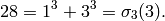
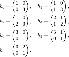
Example 1.55
Next we compute  explicitly.
The Manin symbol generators are
explicitly.
The Manin symbol generators are


The relation matrix is as follows, where the -relations
are above the line and the -relations
are below it:
In weight , two out of three -relations are redundant, so we
do not include them.
The reduced row echelon form of the relation matrix is
From the echelon form we see that every symbol
is equivalent to a combination of
 ,
,  , and
, and  .
(Notice that columns ,
.
(Notice that columns ,  , and
, and  are the pivot
columns, where we index columns starting at .)
are the pivot
columns, where we index columns starting at .)
To compute , we apply each of the Heilbronn
matrices of determinant from Proposition 1.29
to , then to  , and finally to
  .
The matrices are as in Example 1.54 above.
We have
.
The matrices are as in Example 1.54 above.
We have

Applying to , we get

Applying to , we get

Thus the matrix of with respect to this basis is
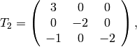
where we write the matrix as an operator on the left on vectors
written in terms of , , and .
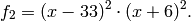
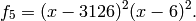
The matrix has characteristic polynomial
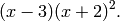
The  factor corresponds to the weight Eisenstein
series, and the
factor corresponds to the weight Eisenstein
series, and the  factor corresponds to the elliptic
curve
factor corresponds to the elliptic
curve  , which has

Example 1.56
In this example, we compute  ,
which illustrates both weight greater than
and level greater than .
We have the following generating Manin symbols:
,
which illustrates both weight greater than
and level greater than .
We have the following generating Manin symbols:
![x_{0} &= [XY^4,(0,1)],\qquad x_{1} = [XY^4,(1,0)],\\
x_{2} &= [XY^4,(1,1)], \qquad x_{3} = [XY^4,(1,2)],\\
x_{4} &= [XY^3,(0,1)], \qquad x_{5} = [XY^3,(1,0)],\\
x_{6} &= [XY^3,(1,1)], \qquad
x_{7} = [XY^3,(1,2)],\\
x_{8} &= [X^2Y^2,(0,1)], \qquad
\!\!x_{9} = [X^2Y^2,(1,0)],\\
x_{10} &= [X^2Y^2,(1,1)], \qquad
\!\!\!\!x_{11} = [X^2Y^2,(1,2)],\\
x_{12} &= [X^3Y,(0,1)], \qquad
x_{13} = [X^3Y,(1,0)],\\
x_{14} &= [X^3Y,(1,1)], \qquad
x_{15} = [X^3Y,(1,2)],\\
x_{16} &= [X^4Y,(0,1)], \qquad
x_{17} = [X^4Y,(1,0)],\\
x_{18} &= [X^4Y,(1,1)], \qquad
x_{19} = [X^4Y,(1,2)].\\](_images/math/c23c748c064afa76e3d39429a3f1d1ebe1719542.png)
The relation matrix is already very large
for  . It is as follows, where the -relations
are before the line and the -relations after it:
. It is as follows, where the -relations
are before the line and the -relations after it:
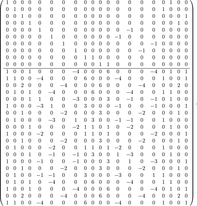
The reduced row echelon form of the relations matrix, with zero rows removed is
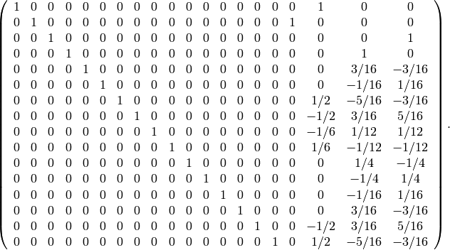
Since these relations are equivalent to the original
relations, we see how
 can be expressed in
terms of
can be expressed in
terms of  ,
,  ,
,  , and
, and  .
Thus has dimension
.
Thus has dimension  .
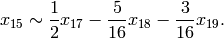
For example,
.
For example,
Notice that the number of relations is already quite large. It is
perhaps surprising how complicated the presentation is already for
. Because there are denominators in the
relations, the above calculation is only a computation of
 . Computing
  involves
finding a -basis for the kernel of the relation matrix
(see Exercise 7.5).
involves
finding a -basis for the kernel of the relation matrix
(see Exercise 7.5).
As before, we find that with respect to the basis
, , , and
Notice that there are denominators in the matrix for
with respect to this basis. It is clear from
the definition of acting on Manin symbols that
preserves the -module ,
so there is some basis for
such that is given by an integer matrix. Thus
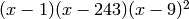
the characteristic polynomial  of will have integer
coefficients; indeed,
of will have integer
coefficients; indeed,
Note the factor  , which comes from the two images
of the Eisenstein series
, which comes from the two images
of the Eisenstein series  of level . The
factor
of level . The
factor  comes from the cusp form

By computing more Hecke operators , we
can find more coefficients of  .
For example, the charpoly of
.
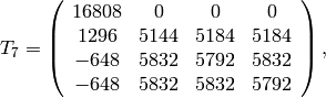
For example, the charpoly of  is
is
 , and the matrix of
  is
is
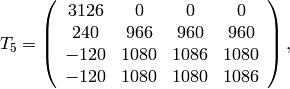
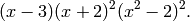
which has characteristic polynomial
The matrix of  is
is
with characteristic polynomial

One can put this information together to deduce that

Example 1.57
Consider  , which has dimension
  .
With respect to the symbols
.
With respect to the symbols

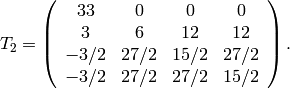
the matrix of is
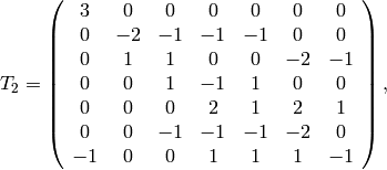
which has characteristic polynomial
There is one Eisenstein series and there are three cusp forms
with  and
and  .
.
Example 1.58
To compute
 , we first make
a list of the
, we first make
a list of the

elements  using Algorithm 1.50.
The list looks like this:
using Algorithm 1.50.
The list looks like this:

For each of the symbols  , we consider the -relations
and -relations.
Ignoring the redundant relations, we find
, we consider the -relations
and -relations.
Ignoring the redundant relations, we find  -relations and
 -relations. It is simple to quotient out by the
-relations, e.g., by identifying with
-relations. It is simple to quotient out by the
-relations, e.g., by identifying with  for
some (or setting
for
some (or setting  if
if  ). Once we have taken
the quotient by the -relations, we take the image of all
of the -relations modulo the -relations and quotient out by
those relations. Because and do not commutate, we cannot
only quotient out by -relations
). Once we have taken
the quotient by the -relations, we take the image of all
of the -relations modulo the -relations and quotient out by
those relations. Because and do not commutate, we cannot
only quotient out by -relations  where
the are the basis after quotienting out by the -relations.
The relation matrix has rank
where
the are the basis after quotienting out by the -relations.
The relation matrix has rank  , so has
dimension
, so has
dimension  .
.
If we instead compute the quotient  of by the subspace of elements
  ,
we include relations
,
we include relations  , where
  .
There are now 2016 -relations, 2024
.
There are now 2016 -relations, 2024  -relations,
and 1344 -relations. Again, it is relatively easy to quotient
out by the -relations by identifying and
-relations,
and 1344 -relations. Again, it is relatively easy to quotient
out by the -relations by identifying and  .
We then take the image of all
.
We then take the image of all  -relations modulo the
-relations, and again directly quotient out by the -relations
by identifying
-relations modulo the
-relations, and again directly quotient out by the -relations
by identifying ![[x_i]](_images/math/487e544a359d32cf1d604be8c662ffb928535bd1.png) with
with ![-[x_iI]=-[x_j]](_images/math/0db15655aa8691e5c33046015df3730d3a4a76fe.png) for some , where
by we mean the class of modulo the -relations.
Finally, we quotient out by the -relations, which involves
sparse Gauss elimination on a matrix with rows
and at most three nonzero entries per row.
The dimension of is
for some , where
by we mean the class of modulo the -relations.
Finally, we quotient out by the -relations, which involves
sparse Gauss elimination on a matrix with rows
and at most three nonzero entries per row.
The dimension of is  .
.
Refined Algorithm for the Presentation
Algorithm 1.59
This is an algorithm to compute  or
or
 , which
only requires doing generic sparse linear algebra to deal
with the three term -relations.
, which
only requires doing generic sparse linear algebra to deal
with the three term -relations.
Let
 by a list of all Manin symbols.
Quotient out the two-term
-relations and if the  quotient is desired, by the two-term
  -relations.
(Note that this is more subtle than
just “identifying symbols in pairs”,
since complicated relations can cause generators to surprisingly
equal .)
Let denote the class of after this quotienting
process.
-relations.
(Note that this is more subtle than
just “identifying symbols in pairs”,
since complicated relations can cause generators to surprisingly
equal .)
Let denote the class of after this quotienting
process.Create a sparse matrix
with  columns, whose rows
encode the relations
columns, whose rows
encode the relations![[x_i] + [x_iT] + [x_iT^2] = 0.](_images/math/f05aefe6b28554d38ddb235662923d34e8667ff7.png)
For example, there are about
 such rows when
.
The number of nonzero entries per row is at most
such rows when
.
The number of nonzero entries per row is at most  .
Note that we must include rows for all , since
even if
.
Note that we must include rows for all , since
even if ![[x_i] = [x_j]](_images/math/c0a83ea46386d0ca4de420a7027e6e01c33c1e7d.png) , it need not be the case that
, it need not be the case that
![[x_i T] = [x_jT]](_images/math/55465c71c6bbd80a9d32d036ebde7f2d2fbd7ef5.png) , since the matrices and do not commute.
However, we have an a priori formula for the dimension
of the quotient by all these relations, so we could omit
many relations and just check that there are enough at the
end—if there are not, we add in more.
, since the matrices and do not commute.
However, we have an a priori formula for the dimension
of the quotient by all these relations, so we could omit
many relations and just check that there are enough at the
end—if there are not, we add in more.Compute the reduced row echelon form of
using
Algorithm 7.6. For , this is the echelon
form of a matrix with size about  .
.Use what we have done above to read off a sparse matrix
that expresses each of the Manin symbols in terms of
a basis of Manin symbols, modulo the relations.
Applications
Later in This Book
We sketch some of the ways in which we will apply the modular symbols algorithms of this chapter later in this book.
Cuspidal modular symbols are in Hecke-equivariant duality with
cuspidal modular forms, and as such we can compute modular forms by
computing systems of eigenvalues for the Hecke operators acting on
modular symbols. By the Atkin-Lehner-Li theory of newforms (see,
e.g., Theorem 9.4), we can construct  for
any , any , and using this method. See
Chapter Modular Forms for more details.
for
any , any , and using this method. See
Chapter Modular Forms for more details.
Once we can compute spaces of modular symbols, we move to computing
the corresponding modular forms. We
define inclusion and trace maps from modular symbols of one level
to modular symbols of level a multiple or divisor of . Using these,
we compute the quotient of the new subspace of cuspidal modular
symbols on which a “star involution” acts as . The Hecke
operators act by diagonalizable commuting matrices on this space, and
computing the systems of Hecke eigenvalues is equivalent
to computing newforms  . In this way, we
obtain a list of all newforms (normalized eigenforms) in
for any , , and .
. In this way, we
obtain a list of all newforms (normalized eigenforms) in
for any , , and .
In Chapter Computing Periods, we compute with the period mapping from
modular symbols to  attached to a newform
  .
When
.
When  and has rational Fourier coefficients, this
gives a method to compute the period lattice associated to a modular
elliptic curve attached to a newform (see
Section All Elliptic Curves of Given Conductor). In general, computation of this map
is important when finding equations for modular -curves, CM
curves, and curves with a given modular Jacobian. It is also
important for computing special values of the -function at
integer points in the critical strip.
and has rational Fourier coefficients, this
gives a method to compute the period lattice associated to a modular
elliptic curve attached to a newform (see
Section All Elliptic Curves of Given Conductor). In general, computation of this map
is important when finding equations for modular -curves, CM
curves, and curves with a given modular Jacobian. It is also
important for computing special values of the -function at
integer points in the critical strip.
Discussion of the Literature and Research
Modular symbols were introduced by Birch [Bir71] for
computations in support of the Birch and Swinnerton-Dyer conjecture.
Manin [Man72] used modular symbols to
prove rationality results about special values of -functions.
Merel’s paper [Mer94] builds on work of Shokurov (mainly
[Sho80a]), which develops a higher-weight
generalization of Manin’s work partly to understand rationality
properties of special values of -functions. Cremona’s book
[Cre97a] discusses how to compute the space of
weight modular symbols for , in connection with the
problem of enumerating all elliptic curves of given conductor, and his
article [Cre92] discusses the case and
computation of modular symbols with character.
There have been several Ph.D. theses about modular symbols.
Basmaji’s thesis [Bas96] contains tricks to efficiently
compute Hecke operators , with very large (see
Section Basmaji’s Trick), and also discusses how to compute spaces
of half integral weight modular forms building on what one can get
from modular symbols of integral weight. The author’s Ph.D. thesis
[Ste00] discusses higher-weight modular
symbols and applies modular symbols to study Shafarevich-Tate groups
(see also [Aga00]). Martin’s thesis [Mar01] is
about an attempt to study an analogue of analytic modular symbols for
weight . Gabor Wiese’s thesis [Wie05] uses modular
symbols methods to study weight 1 modular forms modulo . Lemelin’s
thesis [Lem01] discusses modular symbols for quadratic
imaginary fields in the context of -adic analogues of the Birch and
Swinnerton-Dyer conjecture. See also the survey paper
[FM99], which discusses computation with weight
modular symbols in the context of modular abelian
varieties.
The appendix of this book is about
analogues of modular symbols for groups besides
finite index subgroups of , e.g., for subgroup
of higher rank groups such as  .
There has also been work on computing Hilbert
modular forms, e.g., by Lassina Dembel’e [Dem05] Hilbert modular forms are functions on a product of copies of , and
is replaced by a group of matrices with entries in a
totally real field.
.
There has also been work on computing Hilbert
modular forms, e.g., by Lassina Dembel’e [Dem05] Hilbert modular forms are functions on a product of copies of , and
is replaced by a group of matrices with entries in a
totally real field.
Glenn Stevens, Robert Pollack and Henri Darmon (see
[DP04]) have worked for many years to develop an
analogue of modular symbols in a rigid analytic context, which is
helpful for questions about computing with overconvergent
-adic modular forms or proving results about -adic
-functions.
Finally we mention that Barry Mazur and some other authors
use the term “modular symbol”
in a different way than we do.
They use the term in a way that is dual
to our usage; for example, they attach a “modular symbol” to
a modular form or elliptic curve.
See [MTT86] for an extensive discussion
of modular symbols from this point of view, where they are used to
construct -adic -functions.
Exercises
Exercise 1.11
Suppose is an integer multiple of . Prove
that the natural map  is surjective.
Exercise 1.12
Prove that  is surjective
(see Lemma 1.36).
is surjective
(see Lemma 1.36).
Exercise 1.13
Compute  . List
each Manin symbol the relations they satisfy, compute
the quotient, etc. Find the matrix of .
(Check: The dimension of is , and
the characteristic polynomial of is
. List
each Manin symbol the relations they satisfy, compute
the quotient, etc. Find the matrix of .
(Check: The dimension of is , and
the characteristic polynomial of is  .)
.)
Exercise 1.14
Finish the proof of Proposition 1.38.
Exercise 1.15
- Show that if
 , then
 for
and .
for
and . - (*) Give an example of a finite index
subgroup such that
 .
.
Table Of Contents
- General Modular Symbols