A Proof of Quadratic Reciprocity Using Gauss Sums

In this section we present a beautiful proof of Theorem 4.1.7 using algebraic identities satisfied by sums of ``roots of unity''. The objects we introduce in the proof are of independent interest, and provide a powerful tool to prove higher-degree analogues of quadratic reciprocity. (For more on higher reciprocity see [#!ireland-rosen!#]. See also Section 6 of [#!ireland-rosen!#] on which the proof below is modeled.)

Definition 4.4 (Root of Unity)   An $n$ th root of unity is a complex number $\zeta$ such that $\zeta^n=1$ . A root of unity $\zeta$ is a primitive $n$ th root of unity if $n$ is the smallest positive integer such that $\zeta^n=1$ .

For example, $-1$ is a primitive second root of unity, and $\zeta = \frac{\sqrt{-3}-1}{2}$ is a primitive cube root of unity. More generally, for any $n\in\mathbb{N}$ the complex number

$$\zeta_n =\cos(2\pi{} /n) + i \sin(2\pi{}/n)$$

is a primitive $n$ th root of unity (this follows from the identity $e^{i\theta} = \cos(\theta) + i\sin(\theta)$ ). For the rest of this section, we fix an odd prime $p$ and the primitive $p$ th root  $\zeta=\zeta_p$ of unity.

SAGE Example 4.4   In SAGE use the CyclotomicField command to create an exact $p$ th root of $\zeta$ unity. Expressions in $\zeta$ are always re-expressed as polynomials in $\zeta$ of degree at most $p-1$ .

sage: K.<zeta> = CyclotomicField(5)
sage: zeta^5
1
sage: 1/zeta
-zeta^3 - zeta^2 - zeta - 1

Definition 4.4 (Gauss Sum)   Fix an odd prime $p$ . The Gauss sum associated to an integer $a$ is

$$g_a = \sum_{n=0}^{p-1} \left(\frac{n}{p}\right) \zeta^{an},$$

where $\zeta=\zeta_p = \cos(2\pi{} /p) + i \sin(2\pi{}/p)$ .

Note that $p$ is implicit in the definition of $g_a$ . If we were to change $p$ , then the Gauss sum $g_a$ associated to $a$ would be different. The definition of $g_a$ also depends on our choice of $\zeta$ ; we've chosen $\zeta=\zeta_p$ , but could have chosen a different $\zeta$ and then $g_a$ could be different.

SAGE Example 4.4   We define in SAGE a function gauss_sum and compute the Gauss sum $g_2$ for $p=5$ :

sage: def gauss_sum(a,p): 
...   K.<zeta> = CyclotomicField(p)
...   return sum(legendre_symbol(n,p) * zeta^(a*n) for n in range(p))
sage: g2 = gauss_sum(2,5); g2
2*zeta^3 + 2*zeta^2 + 1
sage: g2.complex_embedding()
-2.23606797749979 + 0.000000000000000333066907387547*I
sage: g2^2 
5

Here $g_2$ is initially output as a polynomial in $\zeta_5$ , so there is no loss of precision. The complex_embedding command shows some embedding of $g_2$ into the complex numbers, which is only correct to about the first 15 digits. Note that $g_2^2 = 5$ , so $g_2 = -\sqrt{5}$ .

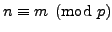
Figure 4.1: Gauss sum $g_2$ for $p=5$

Figure 4.1 illustrates the Gauss sum $g_2$ for $p=5$ . The Gauss sum is obtained by adding the points on the unit circle, with signs as indicated, to obtain the real number $-\sqrt{5}$ . This suggests the following proposition, whose proof will require some work.

Proposition 4.4 (Gauss sum)   For any $a$ not divisible by $p$ ,

$$\displaystyle g_a^2 = (-1)^{(p-1)/2}p.$$

SAGE Example 4.4   We illustrate using SAGE that the proposition is correct for $p=7$ and $p=13$ :

sage: [gauss_sum(a, 7)^2 for a in range(1,7)] 
[-7, -7, -7, -7, -7, -7]
sage: [gauss_sum(a, 13)^2 for a in range(1,13)]  
[13, 13, 13, 13, 13, 13, 13, 13, 13, 13, 13, 13]

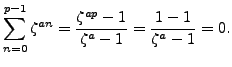
In order to prove the proposition, we introduce a few lemmas.

Lemma 4.4   For any integer $a$ ,

$$\sum_{n=0}^{p-1} \zeta^{an} = \begin{cases} p & \text{\rm if $a \equiv 0\pmod{p}$,}\\ 0 & \text{\rm otherwise.} \end{cases}$$

Proof. If $a\equiv 0\pmod{p}$ , then $\zeta^a=1$ , so the sum equals the number of summands, which is $p$ . If $a\not\equiv 0\pmod{p}$ , then we use then identity

$$x^p - 1 = (x-1)(x^{p-1} + \cdots + x + 1)$$

with $x = \zeta^a$ . We have $\zeta^a\neq 1$ , so $\zeta^a - 1 \neq 0$ and

$$\sum_{n=0}^{p-1} \zeta^{an} = \frac{\zeta^{ap}-1}{\zeta^a-1} = \frac{1-1}{\zeta^a-1} = 0.$$

$\qedsymbol$

Lemma 4.4   If $x$ and $y$ are arbitrary integers, then

$$\sum_{n=0}^{p-1} \zeta^{(x-y)n} = \begin{cases} p & \text{\... ... $x\equiv y\pmod{p}$},\\ 0 & \text{\rm otherwise}. \end{cases}$$

Proof. This follows from Lemma 4.4.7 by setting $a=x-y$ . $\qedsymbol$

Lemma 4.4   We have $g_0=0$ .

Proof. By definition

$$g_0 = \sum_{n=0}^{p-1} \left(\frac{n}{p}\right).$$ (4.4.1)

By Lemma 4.1.4, the map

$$\left(\frac{\cdot}{p}\right) : (\mathbb{Z}/p\mathbb{Z}{})^* \rightarrow \{\pm 1\}$$

is a surjective homomorphism of groups. Thus half the elements of $(\mathbb{Z}/p\mathbb{Z}{})^*$ map to $+1$ and half map to $-1$ (the subgroup that maps to $+1$ has index $2$ ). Since $\left(\frac{0}{p}\right)=0$ , the sum (4.4.1) is 0 . $\qedsymbol$

Lemma 4.4   For any integer $a$ ,

$$g_a = \left(\frac{a}{p}\right)g_1.$$

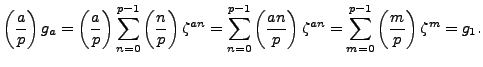
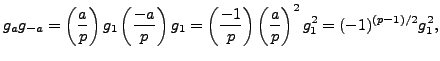
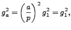
Proof. When $a\equiv 0\pmod{p}$ the lemma follows from Lemma 4.4.9, so suppose that $a\not\equiv 0\pmod{p}$ . Then

$$\left(\frac{a}{p}\right) g_a = \left(\frac{a}{p}\right) \sum_{n=0... ...}\right) \zeta^{an} = \sum_{m=0}^{p-1}\left(\frac{m}{p}\right)\zeta^{m} = g_1.$$

Here we use that multiplication by $a$ is an automorphism of $\mathbb{Z}/p\mathbb{Z}{}$ . Finally, multiply both sides by $\left(\frac{a}{p}\right)$ and use that $\left(\frac{a}{p}\right)^2=1$ . $\qedsymbol$

We have enough lemmas to prove Proposition 4.4.5.

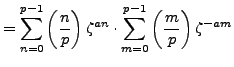
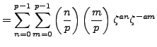
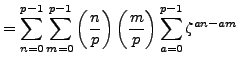
Proof. [Proof of Proposition 4.4.5] We evaluate the sum $\sum_{a=0}^{p-1} g_a g_{-a}$ in two different ways. By Lemma 4.4.10, since $a\not\equiv 0\pmod{p}$ we have

$$g_a g_{-a} = \left(\frac{a}{p}\right)g_1\left(\frac{-a}{p}\right)... ...ft(\frac{-1}{p}\right)\left(\frac{a}{p}\right)^2 g_1^2 = (-1)^{(p-1)/2} g_1^2,$$

where the last step follows from Proposition 4.2.1 and that $\left(\frac{a}{p}\right)\in\{\pm 1\}$ . Thus

$$\sum_{a=0}^{p-1} g_a g_{-a} = (p-1)(-1)^{(p-1)/2}g_1^2.$$ (4.4.2)

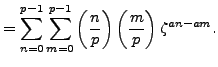
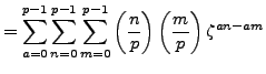
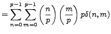
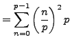
On the other hand, by definition

$$g_a g_{-a} = \sum_{n=0}^{p-1} \left(\frac{n}{p}\right)\zeta^{an} \cdot \sum_{m=0}^{p-1}\left(\frac{m}{p}\right)\zeta^{-am}$$

$$= \sum_{n=0}^{p-1}\sum_{m=0}^{p-1} \left(\frac{n}{p}\right)\left(\frac{m}{p}\right)\zeta^{an}\zeta^{-am}$$

$$= \sum_{n=0}^{p-1}\sum_{m=0}^{p-1} \left(\frac{n}{p}\right)\left(\frac{m}{p}\right)\zeta^{an-am}.$$

Let $\delta(n,m)=1$ if $n\equiv m\pmod{p}$ and 0 otherwise. By Lemma 4.4.8,

$$\sum_{a=0}^{p-1} g_a g_{-a} = \sum_{a=0}^{p-1}\sum_{n=0}^{p-1}\sum_{m=0}^{p-1} \left(\frac{n}{p}\right)\left(\frac{m}{p}\right)\zeta^{an-am}$$

$$= \sum_{n=0}^{p-1}\sum_{m=0}^{p-1} \left(\frac{n}{p}\right)\left(\frac{m}{p}\right)\sum_{a=0}^{p-1}\zeta^{an-am}$$

$$= \sum_{n=0}^{p-1}\sum_{m=0}^{p-1} \left(\frac{n}{p}\right)\left(\frac{m}{p}\right)p\delta(n,m)$$

$$= \sum_{n=0}^{p-1}\left(\frac{n}{p}\right)^2 p$$

$$= p(p-1).$$

Equate (4.4.2) and the above equality, then cancel $(p-1)$ to see that

$$g_1^2 =(-1)^{(p-1)/2} p.$$

Since $a\not\equiv 0\pmod{p}$ , we have $\left(\frac{a}{p}\right)^2=1$ , so by Lemma 4.4.10,

$$g_a^2 = \left(\frac{a}{p}\right)^2 g_1^2 = g_1^2,$$

and the proposition is proved. $\qedsymbol$