Elliptic Curves¶

Cremona’s Databases¶

Cremona’s databases of elliptic curves is part of Sage. The curves up to conductor 10,000 come standard with Sage, and an optional 75MB download gives all his tables up to conductor 130,000. Type sage -i database cremona ellcurve-20071019 to automatically download and install this extended table.

To use the database, just create a curve by giving

sage: EllipticCurve('5077a1')
Elliptic Curve defined by y^2 + y = x^3 - 7*x + 6 over Rational Field
sage: C = CremonaDatabase()
sage: C.number_of_curves()
847550
sage: C[37]
{'a': {'a1': [[0, 0, 1, -1, 0], 1, 1],
       'b1': [[0, 1, 1, -23, -50], 0, 3], ...
sage: C.isogeny_class('37b')
[Elliptic Curve defined by y^2 + y = x^3 + x^2 - 23*x - 50
over Rational Field, ...]

There is also a Stein-Watkins database that contains hundreds of millions of elliptic curves. It’s over a 2GB download though!

Bryan Birch’s Birthday Card¶

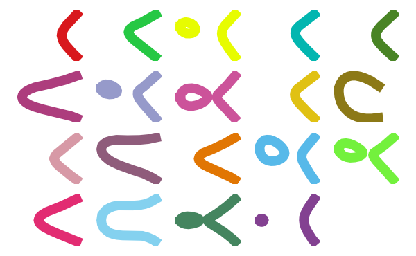
Bryan Birch’s recently had a birthday conference, and I used Sage to draw the cover of his birthday card by enumerating all optimal elliptic curves of conductor up to 37, then plotting them with thick randomly colored lines. As you can see below, plotting an elliptic curve is as simple as calling the plot method on it. Also, the graphics array command allows us to easily combine numerous plots into a single graphics object.

sage: v = cremona_optimal_curves([11..37])
sage: w = [E.plot(thickness=10,
   rgbcolor=(random(),random(),random())) for E in v]
sage: graphics_array(w, 4, 5).show(axes=False)

Plotting Modulo $p$ ¶

We can use Sage’s interact feature to draw a plot of an elliptic curve modulo $p$ , with a slider that one drags to change the prime $p$ . The interact feature of Sage is very helpful for interactively changing parameters and viewing the results. Type interact? for more help and examples and visit the webpage http://wiki.sagemath.org/interact.

In the code below we first define the elliptic curve $E$ using the Cremona label 37a. Then we define an interactive function $f$ , which is made interactive using the @interact Python decorator. Because the default for $p$ is primes(2,500), the Sage notebook constructs a slider that varies over the primes up to $500$ . When you drag the slider and let go, a plot is drawn of the affine $\mathbb{F}_p$ points on the curve $E_{\mathbb{F}_p}$ . Of course, one should never plot curves over finite fields, which makes this even more fun.

E = EllipticCurve('37a')
@interact
def f(p=primes(2,500)):
    show(plot(E.change_ring(GF(p)),pointsize=30),
    axes=False, frame=True, gridlines="automatic",
    aspect_ratio=1, gridlinesstyle={'rgbcolor':(0.7,0.7,0.7)})

Schoof-Elkies-Atkin Point Counting¶

Sage includes sea.gp, which is a fast implementation of the SEA (Schoff-Elkies-Atkin) algorithm for counting the number of points on an elliptic curve over $\mathbb{F}_p$ .

We create the finite field $k=\mathbb{F}_{p}$ , where $p$ is the next prime after $10^{20}$ . The next prime command uses Pari’s nextprime function, but proves primality of the result (unlike Pari which gives only the next probable prime after a number). Sage also has a next probable prime function.

sage: k = GF(next_prime(10^20))

compute its cardinality, which behind the scenes uses SEA.

sage: E = EllipticCurve(k.random_element())
sage: E.cardinality()                   # less than a second
100000000005466254167

To see how Sage chooses when to use SEA versus other methods, type E.cardinality?? and read the source code. As of this writing, it simply uses SEA whenever $p>10^{18}$ .

$p$ -adic Regulators¶

Sage has the world’s best code for computing $p$ -adic regulators of elliptic curves, thanks to work of David Harvey and Robert Bradshaw. The $p$ -adic regulator of an elliptic curve $E$ at a good ordinary prime $p$ is the determinant of the global $p$ -adic height pairing matrix on the Mordell-Weil group $E(\mathbb{Q})$ . (This has nothing to do with local or archimedean heights.) This is the analogue of the regulator in the Mazur-Tate-Teitelbaum $p$ -adic analogue of the Birch and Swinnerton-Dyer conjecture.

In particular, Sage implements Harvey’s improvement on an algorithm of Mazur-Stein-Tate, which builds on Kiran Kedlaya’s Monsky-Washnitzer approach to computing $p$ -adic cohomology groups.

We create the elliptic curve with Cremona label 389a, which is the curve of smallest conductor and rank $2$ . We then compute both the $5$ -adic and $997$ -adic regulators of this curve.

sage: E = EllipticCurve('389a')
sage: E.padic_regulator(5, 10)
5^2 + 2*5^3 + 2*5^4 + 4*5^5 + 3*5^6 + 4*5^7 + 3*5^8 + 5^9 + O(5^11)
sage: E.padic_regulator(997, 10)
740*997^2 + 916*997^3 + 472*997^4 + 325*997^5 + 697*997^6
          + 642*997^7 + 68*997^8 + 860*997^9 + 884*997^10 + O(997^11)

Before the new algorithm mentioned above, even computing a $7$ -adic regulator to $3$ digits of precision was a nontrivial computational challenge. Now in Sage computing the $100003$ -adic regulator is routine:

sage: E.padic_regulator(100003,5)  # a couple of seconds
42582*100003^2 + 35250*100003^3 + 12790*100003^4 + 64078*100003^5 + O(100003^6)

$p$ -adic $L$ -functions¶

$p$ -adic $L$ -functions play a central role in the arithmetic study of elliptic curves. They are $p$ -adic analogues of complex analytic $L$ -function, and their leading coefficient (at $0$ ) is the analogue of $L^{(r)}(E,1)/\Omega_E$ in the $p$ -adic analogue of the Birch and Swinnerton-Dyer conjecture. They also appear in theorems of Kato, Schneider, and others that prove partial results toward $p$ -adic BSD using Iwasawa theory.

The implementation in Sage is mainly due to work of myself, Christian Wuthrich, and Robert Pollack. We use Sage to compute the $5$ -adic $L$ -series of the elliptic curve 389a of rank $2$ .

sage: E = EllipticCurve('389a')
sage: L = E.padic_lseries(5)
sage: L
5-adic L-series of Elliptic Curve defined
by y^2 + y = x^3 + x^2 - 2*x over Rational Field
sage: L.series(3)
O(5^5) + O(5^2)*T + (4 + 4*5 + O(5^2))*T^2 +
(2 + 4*5 + O(5^2))*T^3 + (3 + O(5^2))*T^4 + O(T^5)

Bounding Shafarevich-Tate Groups¶

Sage implements code to compute numerous explicit bounds on Shafarevich-Tate Groups of elliptic curves. This functionality is only available in Sage, and uses results Kolyvagin, Kato, Perrin-Riou, etc., and unpublished papers of Wuthrich and me.

sage: E = EllipticCurve('11a1')
sage: E.sha().bound()           # so only 2,3,5 could divide sha
[2, 3, 5]
sage: E = EllipticCurve('37a1')  # so only 2 could divide sha
sage: E.sha().bound()
([2], 1)
sage: E = EllipticCurve('389a1')
sage: E.sha().bound()
(0, 0)

The $(0,0)$ in the last output above indicates that the Euler systems results of Kolyvagin and Kato give no information about finiteness of the Shafarevich-Tate group of the curve $E$ . In fact, it is an open problem to prove this finiteness, since $E$ has rank $2$ , and finiteness is only known for elliptic curves for which $L(E,1)\neq 0$ or $L'(E,1)\neq 0$ .

Partial results of Kato, Schneider and others on the $p$ -adic analogue of the BSD conjecture yield algorithms for bounding the $p$ -part of the Shafarevich-Tate group. These algorithms require as input explicit computation of $p$ -adic $L$ -functions, $p$ -adic regulators, etc., as explained in Stein-Wuthrich. For example, below we use Sage to prove that $5$ and $7$ do not divide the Shafarevich-Tate group of our rank $2$ curve 389a.

sage: E = EllipticCurve('389a1')
sage: sha = E.sha()
sage: sha.p_primary_bound(5)  # iwasawa theory ==> 5 doesn't divide sha
0
sage: sha.p_primary_bound(7)  # iwasawa theory ==> 7 doesn't divide sha
0

This is consistent with the Birch and Swinnerton-Dyer conjecture, which predicts that the Shafarevich-Tate group is trivial. Below we compute this predicted order, which is the floating point number $1.000000$ to some precision. That the result is a floating point number helps emphasize that it is an open problem to show that the conjectural order of the Shafarevich-Tate group is even a rational number in general!

sage: E.sha().an()
1.00000000000000

Mordell-Weil Groups and Integral Points¶

Sage includes both Cremona’s mwrank library and Simon’s 2-descent GP scripts for computing Mordell-Weil groups of elliptic curves.

sage: E = EllipticCurve([1,2,5,7,17])
sage: E.conductor()       # not in the Tables
154907
sage: E.gens()            # a few seconds
[(1 : 3 : 1), (67/4 : 507/8 : 1)]

Sage can also compute the torsion subgroup, isogeny class, determine images of Galois representations, determine reduction types, and includes a full implementation of Tate’s algorithm over number fields.

Sage has the world’s fastest implementation of computation of all integral points on an elliptic curve over $\mathbb{Q}$ , due to work of Cremona, Michael Mardaus, and Tobias Nagel. This is also the only free open source implementation available.

sage: E = EllipticCurve([1,2,5,7,17])
sage: E.integral_points(both_signs=True)
[(1 : -9 : 1), (1 : 3 : 1)]

A very impressive example is the lowest conductor elliptic curve of rank $3$ , which has 36 integral points.

sage: E = elliptic_curves.rank(3)[0]
sage: E.integral_points(both_signs=True)   # less than 3 seconds
[(-3 : -1 : 1), (-3 : 0 : 1), (-2 : -4 : 1), (-2 : 3 : 1),
 ...(816 : -23310 : 1), (816 : 23309 : 1)]

The algorithm to compute all integral points involves first computing the Mordell-Weil group, then bounding the integral points, and listing all integral points satisfying those bounds. See Cohen’s new GTM 239 for complete details.

The complexity grows exponentially in the rank of the curve. We can do the above calculation, but with the first known curve of rank $4$ , and it finishes in about a minute (and outputs 64 points).

sage: E = elliptic_curves.rank(4)[0]
sage: E.integral_points(both_signs=True)   # about a minute
[(-10 : 3 : 1), (-10 : 7 : 1), ...
 (19405 : -2712802 : 1), (19405 : 2693397 : 1)]

$L$ -functions¶

Evaluation¶

We next compute with the complex $L$ -function

$L(E,s) = \prod_{p\nmid \Delta=389} \frac{1}{1-a_p p^{-s} + p p^{-2s}} \cdot \prod_{p\mid \Delta=389} \frac{1}{1-a_p p^{-s}}$

of $E$ . Though the above Euler product only defines an analytic function on the right half plane where $\text{Re}(s) > 3/2$ , a deep theorem of Wiles et al. (the Modularity Theorem) implies that it has an analytic continuation to the whole complex plane and functional equation. We can evaluate the function $L$ anywhere on the complex plane using Sage (via code of Tim Dokchitser).

sage: E = EllipticCurve('389a1')
sage: L = E.lseries()
sage: L
Complex L-series of the Elliptic Curve defined by
       y^2 + y = x^3 + x^2 - 2*x over Rational Field
sage: L(1)
-1.04124792770327e-19
sage: L(1+I)
-0.638409938588039 + 0.715495239204667*I
sage: L(100)
1.00000000000000

Taylor Series¶

We can also compute the Taylor series of $L$ about any point, thanks to Tim Dokchitser’s code.

sage: E = EllipticCurve('389a1')
sage: L = E.lseries()
sage: Ld = L.dokchitser()
sage: Ld.taylor_series(1,4)
-1.28158145691931e-23 + (7.26268290635587e-24)*z + 0.759316500288427*z^2
                      - 0.430302337583362*z^3 + O(z^4)

GRH¶

The Generalized Riemann Hypothesis asserts that all nontrivial zeros of $L(E,s)$ are of the form $1+iy$ . Mike Rubinstein has written a C++ program that is part of Sage that can for any $n$ compute the first $n$ values of $y$ such that $1+iy$ is a zero of $L(E,s)$ . It also verifies the Riemann Hypothesis for these zeros (I think). Rubinstein’s program can also do similar computations for a wide class of $L$ -functions, though not all of this functionality is as easy to use from Sage as for elliptic curves. Below we compute the first $10$ zeros of $L(E,s)$ , where $E$ is still the rank $2$ curve 389a.

sage: L.zeros(10)
[0.000000000, 0.000000000, 2.87609907, 4.41689608, 5.79340263,
 6.98596665, 7.47490750, 8.63320525, 9.63307880, 10.3514333]

Elliptic Curves¶

Cremona’s Databases¶

Bryan Birch’s Birthday Card¶

Plotting Modulo $p$ ¶

Schoof-Elkies-Atkin Point Counting¶

$p$ -adic Regulators¶

$p$ -adic $L$ -functions¶

Bounding Shafarevich-Tate Groups¶

Mordell-Weil Groups and Integral Points¶

$L$ -functions¶

Evaluation¶

Taylor Series¶

GRH¶

Table Of Contents

Previous topic

Next topic

This Page

Quick search

Navigation

Elliptic Curves¶

Cremona’s Databases¶

Bryan Birch’s Birthday Card¶

Plotting Modulo ¶

Schoof-Elkies-Atkin Point Counting¶

-adic Regulators¶

-adic -functions¶

Bounding Shafarevich-Tate Groups¶

Mordell-Weil Groups and Integral Points¶

-functions¶

Evaluation¶

Taylor Series¶

GRH¶

Table Of Contents

Previous topic

Next topic

This Page

Quick search

Navigation

Plotting Modulo $p$ ¶

$p$ -adic Regulators¶

$p$ -adic $L$ -functions¶

$L$ -functions¶