Computing with Newforms
In this chapter we pull together results and algorithms from Chapter Modular Forms of Weight 2, Dirichlet Characters, Linear Algebra, and General Modular Symbols and explain how to use linear algebra techniques to compute cusp forms and eigenforms using modular symbols.
We first discuss in Section Dirichlet Character Decomposition how to decompose
 as a direct sum of subspaces corresponding to
Dirichlet characters. Next in Section Atkin-Lehner-Li Theory we state the main
theorems of Atkin-Lehner-Li theory, which
decomposes
as a direct sum of subspaces corresponding to
Dirichlet characters. Next in Section Atkin-Lehner-Li Theory we state the main
theorems of Atkin-Lehner-Li theory, which
decomposes  into subspaces on which the
Hecke operators act diagonalizably with “multiplicity one”.
In Section Computing Cusp Forms we describe two
algorithms for computing modular forms. One algorithm finds
a basis of
into subspaces on which the
Hecke operators act diagonalizably with “multiplicity one”.
In Section Computing Cusp Forms we describe two
algorithms for computing modular forms. One algorithm finds
a basis of  -expansions, and the other computes eigenvalues
of newforms.
-expansions, and the other computes eigenvalues
of newforms.
Dirichlet Character Decomposition
The group  acts on through
diamond-bracket operators
acts on through
diamond-bracket operators  , as follows.
For
, as follows.
For  , define
![f|\dbd{d} = f^{\left[\abcd{a}{b}{c}{d'}\right]_k},](_images/math/5251ec5739f742252c1dc951b32443e1029010a6.png)
where  is congruent to
 . Note that the map
 is surjective (see Exercise 1.12),
so the matrix
is surjective (see Exercise 1.12),
so the matrix  exists.
To prove that
exists.
To prove that  preserves ,
we prove the more general fact that
preserves ,
we prove the more general fact that  is a
normal subgroup of
is a
normal subgroup of

This will imply that preserves
since  .
.
Lemma 9.1
The group is a normal subgroup of  ,
and the quotient
,
and the quotient  is
isomorphic to .
is
isomorphic to .
Proof
See Exercise 9.1.
Alternatively, one can prove that preserves
by showing that  and noting that
is preserved by
and noting that
is preserved by  (see
Remark Remark 9.11).
(see
Remark Remark 9.11).
The diamond-bracket action is the action of
 on . Since
is a finite-dimensional vector space over
on . Since
is a finite-dimensional vector space over  , the
action breaks up as a direct sum of
factors corresponding to the Dirichlet characters
, the
action breaks up as a direct sum of
factors corresponding to the Dirichlet characters  of
modulus
of
modulus  .
.
Proposition 9.2
We have
where

Proof
The linear transformations , for the , all
commute, since acts through the abelian group
. Also, if  is the exponent of
, then
is the exponent of
, then  , so the
matrix of is diagonalizable. It is a standard fact from
linear algebra that any commuting family of diagonalizable linear
transformations is simultaneously diagonalizable (see
Exercise 5.1), so there is a basis
, so the
matrix of is diagonalizable. It is a standard fact from
linear algebra that any commuting family of diagonalizable linear
transformations is simultaneously diagonalizable (see
Exercise 5.1), so there is a basis  for such that all act by diagonal
matrices. The system of eigenvalues of the action of on a fixed
for such that all act by diagonal
matrices. The system of eigenvalues of the action of on a fixed
 defines a Dirichlet character, i.e., each has
the property that
defines a Dirichlet character, i.e., each has
the property that  , for all
and some Dirichlet character
, for all
and some Dirichlet character  . The
for a given
. The
for a given  then span
  , and taken together the
must span .
, and taken together the
must span .
Definition 9.3
If  , we say that is
the character of the modular form
, we say that is
the character of the modular form  .
.
The spaces are a direct sum of subspaces
 and
and  , where is the
subspace of cusp forms, i.e., forms that vanish at all
cusps (elements of
, where is the
subspace of cusp forms, i.e., forms that vanish at all
cusps (elements of  ), and
is the subspace of Eisenstein series, which is the unique
subspace of that is invariant under all Hecke
operators and is such that
), and
is the subspace of Eisenstein series, which is the unique
subspace of that is invariant under all Hecke
operators and is such that
 .
The space can also be defined as the space
spanned by all Eisenstein series of weight
.
The space can also be defined as the space
spanned by all Eisenstein series of weight  and level ,
as defined in Chapter Eisenstein Series and Bernoulli Numbers.
The space can be defined in a third way using the Petersson
inner product (see [Lan95, Section VII.5]).
and level ,
as defined in Chapter Eisenstein Series and Bernoulli Numbers.
The space can be defined in a third way using the Petersson
inner product (see [Lan95, Section VII.5]).
The diamond-bracket operators preserve cusp forms, so
the isomorphism of Proposition 9.2 restricts to an
isomorphism of the corresponding cuspidal subspaces.
We illustrate how to use Sage
to make a table of dimension of
and for  .
.
sage: G = DirichletGroup(13)
sage: G
Group of Dirichlet characters of modulus 13 over
Cyclotomic Field of order 12 and degree 4
sage: dimension_modular_forms(Gamma1(13),2)
13
sage: [dimension_modular_forms(e,2) for e in G]
[1, 0, 3, 0, 2, 0, 2, 0, 2, 0, 3, 0]
Next we do the same for  .
.
sage: G = DirichletGroup(100)
sage: G
Group of Dirichlet characters of modulus 100 over
Cyclotomic Field of order 20 and degree 8
sage: dimension_modular_forms(Gamma1(100),2)
370
sage: v = [dimension_modular_forms(e,2) for e in G]; v
[24, 0, 0, 17, 18, 0, 0, 17, 18, 0, 0, 21, 18, 0, 0, 17,
18, 0, 0, 17, 24, 0, 0, 17, 18, 0, 0, 17, 18, 0, 0, 21,
18, 0, 0, 17, 18, 0, 0, 17]
sage: sum(v)
370
Atkin-Lehner-Li Theory
In Section Degeneracy Maps we defined maps between modular symbols
spaces of different level. There are similar maps between spaces of
cusp forms. Suppose and  are positive integers with
  and that
  is a divisor of
  . Let
. Let
(1)
be the degeneracy map, which is given by  .
There are also maps
.
There are also maps  in the other direction; see
[Lan95, Ch. VIII].
in the other direction; see
[Lan95, Ch. VIII].
The old subspace of , denoted  ,
is the sum of the images of all maps
,
is the sum of the images of all maps  with a proper divisor
of and any divisor of (note that depends on
, , and , so there is a slight abuse of notation).
The new subspace of , which we denote by
with a proper divisor
of and any divisor of (note that depends on
, , and , so there is a slight abuse of notation).
The new subspace of , which we denote by
 , is the intersection
of the kernel of all maps with a proper divisor
of . One can use the Petersson inner product to show
that
, is the intersection
of the kernel of all maps with a proper divisor
of . One can use the Petersson inner product to show
that

Moroever, the new and old subspaces are preserved by all Hecke operators.
Let ![\T = \Z[T_1, T_2, \ldots ]](_images/math/6a9e3fe78b30a2bace2ae1b4f66feb94fe0f9c2d.png) be the commutative polynomial ring
in infinitely many indeterminates
be the commutative polynomial ring
in infinitely many indeterminates  . This
ring acts (via acting as the
. This
ring acts (via acting as the  Hecke operator)
on for every integer . Let
Hecke operator)
on for every integer . Let
 be the subring of generated by the with
 .
.
Theorem 9.4
We have a decomposition
(2)
Each space  is a direct
sum of distinct (nonisomorphic) simple
is a direct
sum of distinct (nonisomorphic) simple  -modules.
Proof
The complete proof is in [Li75]. See also [DS05, Ch. 5] for a beautiful modern treatement of this and related results.
The analogue of Theorem 9.4 with  replaced by
 is also true (this is what was proved in
[AL70]). The analogue for is also valid,
as long as we omit the spaces
is also true (this is what was proved in
[AL70]). The analogue for is also valid,
as long as we omit the spaces  for which
 .
.
Example 9.5
If is prime and  , then
 ,
since
,
since  .
.
One can prove using the Petersson inner product that the
operators on , with , are
diagonalizable. Another result of Atkin-Lehner-Li theory is that the
ring of endomorphisms of generated by all
Hecke operators equals the ring generated by the Hecke operators
with  . This statement need not be true if we do not
restrict to the new subspace, as the following example shows.
. This statement need not be true if we do not
restrict to the new subspace, as the following example shows.
Example 9.6
We have

where each of the spaces  has dimension
  . Thus
 . The Hecke operator
  on
on
 has characteristic polynomial
  ,
which is irreducible. Since
,
which is irreducible. Since  commutes with all Hecke
operators , with
commutes with all Hecke
operators , with  , the subring
  of the Hecke
algebra generated by operators with
of the Hecke
algebra generated by operators with  odd is isomorphic
to
odd is isomorphic
to  (the
(the  scalar matrices). Thus on the full space
, we do not have
scalar matrices). Thus on the full space
, we do not have  . However, on the new subspace
we do have this equality, since the new subspace has dimension
. However, on the new subspace
we do have this equality, since the new subspace has dimension  .
.
Example 9.7
The space  has dimension
  and basis
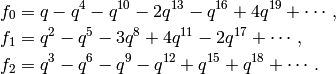
The new subspace  is spanned by the single cusp form

We have  and
and  has dimension with basis

We use Sage to verify the above assertions.
sage: S = CuspForms(Gamma0(45), 2, prec=14); S
Cuspidal subspace of dimension 3 of Modular Forms space
of dimension 10 for Congruence Subgroup Gamma0(45) of
weight 2 over Rational Field
sage: S.basis()
[
q - q^4 - q^10 - 2*q^13 + O(q^14),
q^2 - q^5 - 3*q^8 + 4*q^11 + O(q^14),
q^3 - q^6 - q^9 - q^12 + O(q^14)
]
sage: S.new_subspace().basis()
(q - q^4 - q^10 - 2*q^13 + O(q^14),)
sage: CuspForms(Gamma0(9),2)
Cuspidal subspace of dimension 0 of Modular Forms space
of dimension 3 for Congruence Subgroup Gamma0(9) of
weight 2 over Rational Field
sage: CuspForms(Gamma0(15),2, prec=10).basis()
[
q - q^2 - q^3 - q^4 + q^5 + q^6 + 3*q^8 + q^9 + O(q^10)
]
Example 9.8
This example is similar to Example 9.6, except that there are newforms. We have

where has dimension and
 has dimension .
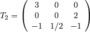
The Hecke operator
has dimension .
The Hecke operator  on
acts via the matrix
on
acts via the matrix
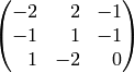
with respect to some basis.
This matrix has eigenvalues and  .
Atkin-Lehner theory asserts that must be a
linear combination of , with
.
Atkin-Lehner theory asserts that must be a
linear combination of , with
 .
Upon computing the matrix for ,
we find by simple linear algebra that
.
Upon computing the matrix for ,
we find by simple linear algebra that  .
.
Definition 9.9
A newform is a -eigenform  that is normalized so that the coefficient of is .
We now motivate this definition by explaining why any -eigenform
can be normalized so that the coefficient of is and how such
an eigenform has the property that its Fourier
coefficients are exactly the Hecke eigenvalues.
Proposition 9.10
If  is an eigenvector for all Hecke operators
normalized so that
is an eigenvector for all Hecke operators
normalized so that  ,
then
,
then  .
.
Proof
If  , then
 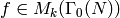 and this
is Lemma 3.22. However, we have not
yet considered Hecke operators on -expansions for
more general spaces of modular forms.
and this
is Lemma 3.22. However, we have not
yet considered Hecke operators on -expansions for
more general spaces of modular forms.
The Hecke operators  , for
, for  prime, act on
by
prime, act on
by
and there is a similar formula for  with
with  composite.
If
composite.
If  is an eigenform for all
, with eigenvalues
is an eigenform for all
, with eigenvalues  , then by the above formula
(3)
Equating coefficients of , we see that if
 , then
  for all ; hence
 for all , because of the multiplicativity of Fourier
coefficients and the recurrence
for all , because of the multiplicativity of Fourier
coefficients and the recurrence
This would mean that  , a contradiction. Thus
  ,
and it makes sense to normalize so that .
With this normalization, (3) implies that
,
and it makes sense to normalize so that .
With this normalization, (3) implies that  ,
as desired.
,
as desired.
Remark 9.11
The Hecke algebra  on contains the
operators , since they satisfy the relation
on contains the
operators , since they satisfy the relation  . Thus any -eigenform in
lies in a subspace for some
Dirichlet character . Also, one can even prove that
. Thus any -eigenform in
lies in a subspace for some
Dirichlet character . Also, one can even prove that
![\dbd{d} \in \Z[\ldots,T_n,\ldots]](_images/math/9dc797ae4ce7b1376dad3999d3a632b593495d6e.png) (see
Exercise 9.2).
(see
Exercise 9.2).
Computing Cusp Forms
Let  be the space of cuspidal modular symbols as in
Chapter General Modular Symbols. Let
be the space of cuspidal modular symbols as in
Chapter General Modular Symbols. Let  be the map of
(?), and let
be the map of
(?), and let  be the plus one quotient of cuspidal modular symbols,
i.e., the quotient of by the image of
be the plus one quotient of cuspidal modular symbols,
i.e., the quotient of by the image of  .
It follows from
Theorem 1.44 and compatibility of the
degeneracy maps (for modular symbols they are defined
in Section Degeneracy Maps) that the -modules
.
It follows from
Theorem 1.44 and compatibility of the
degeneracy maps (for modular symbols they are defined
in Section Degeneracy Maps) that the -modules  and
and  are dual as -modules.
Thus finding the systems of -eigenvalues on cusp forms is the same
as finding the systems of -eigenvalues on cuspidal modular
symbols.
are dual as -modules.
Thus finding the systems of -eigenvalues on cusp forms is the same
as finding the systems of -eigenvalues on cuspidal modular
symbols.
Our strategy to compute is to first compute spaces
using the Atkin-Lehner-Li decomposition
(2). To compute to a given
precision, we compute the systems of eigenvalues of the Hecke
operators on the space  , which we
will define below. Using Proposition 9.10, we then
recover a basis of -expansions for newforms. Note that we only
need to compute Hecke eigenvalues , for prime, not the
for composite, since the
, which we
will define below. Using Proposition 9.10, we then
recover a basis of -expansions for newforms. Note that we only
need to compute Hecke eigenvalues , for prime, not the
for composite, since the  can be quickly recovered in terms
of the
can be quickly recovered in terms
of the  using multiplicativity and the recurrence.
For some problems, e.g., construction of models for modular curves,
having a basis of -expansions is enough. For many other problems,
e.g., enumeration of modular abelian varieties, one is really
interested in the newforms. We next discuss algorithms aimed at each
of these problems.
A Basis of -Expansions
The following algorithm generalizes Algorithm 3.26.
It computes without finding any eigenspaces.
Algorithm 9.12
Given integers , and and a Dirichlet character with
modulus , this algorithm computes a basis of -expansions
for to precision  .
.
[Compute Modular Symbols] Use Algorithm 1.59 to compute
viewed as a
 vector space,
with an action of the .
vector space,
with an action of the .[Basis for Linear Dual] Write down a basis for
 . E.g., if we identify
 with
with  viewed as column vectors, then
  is the space
of row vectors of length , and the pairing is the row
is the space
of row vectors of length , and the pairing is the row  column product.
[Find Generator] Find
 such that
 by choosing random
  until we find
one that generates. The set of that fail
to generate lie in a union of a finite number of
proper subspaces.
until we find
one that generates. The set of that fail
to generate lie in a union of a finite number of
proper subspaces.[Compute Basis] The set of power series
forms a basis for
to precision .
In practice Algorithm 9.12 seems slower than the
eigenspace algorithm that we will describe in the rest of this
chapter. The theoretical complexity of Algorithm 9.12
may be better, because it is not necessary to factor any
polynomials. Polynomial factorization is difficult from the worst-case
complexity point of view, though it is usually fast in practice. The
eigenvalue algorithm only requires computing a few images  for
prime and a Manin symbol on which can easily be
computed. The Merel algorithm involves computing
for
prime and a Manin symbol on which can easily be
computed. The Merel algorithm involves computing  for
all and for a fairly easy , which is potentially more work.
for
all and for a fairly easy , which is potentially more work.
Remark 9.13
By “easy “, I mean that computing is easier on
than on a completely random element of  ,
e.g., could be a Manin symbol.
,
e.g., could be a Manin symbol.
Newforms: Systems of Eigenvalues
In this section we describe an algorithm for computing the system of Hecke eigenvalues associated to a simple subspace of a space of modular symbols. This algorithm is better than doing linear algebra directly over the number field generated by the eigenvalues. It only involves linear algebra over the base field and also yields a compact representation for the answer, which is better than writing the eigenvalues in terms of a power basis for a number field. In order to use this algorithm, it is necessary to decompose the space of cuspidal modular symbols as a direct sum of simples, e.g., using Algorithm 7.17.
Fix and a Dirichlet character of modulus ,
and let
be the  quotient of
modular symbols (see equation (?)).
quotient of
modular symbols (see equation (?)).
Algorithm 9.14
Given a -simple subspace  of modular symbols, this
algorithm outputs maps
of modular symbols, this
algorithm outputs maps  and , where
  is a
is a  -linear map and
  is an isomorphism of
  with
a number field
with
a number field  , such that
  is the
eigenvalue of the Hecke operator acting on a fixed
-eigenvector in
is the
eigenvalue of the Hecke operator acting on a fixed
-eigenvector in  . (Thus
 is a newform.)
[Compute Projection] Let
 be any surjective linear map
such that
be any surjective linear map
such that  equals the kernel
of the -invariant projection onto .
For example, compute
equals the kernel
of the -invariant projection onto .
For example, compute  by finding a simple submodule
of
by finding a simple submodule
of  that is isomorphic to , e.g., by applying
Algorithm 7.17 to with
that is isomorphic to , e.g., by applying
Algorithm 7.17 to with  replaced by
the transpose of .
replaced by
the transpose of .[Choose
 ]label{step:eig:v} Choose a nonzero element
 such that
  and computation of
  is
“easy”, e.g., choose to be a Manin symbol.
is
“easy”, e.g., choose to be a Manin symbol.[Map from Hecke Ring] Let
be the map  , given
by
, given
by  . Note that computation of
is relatively easy, because was chosen so that
. Note that computation of
is relatively easy, because was chosen so that
 is relatively easy to compute. In particular,
if
is relatively easy to compute. In particular,
if  , we do not need to compute the full matrix
of on ; instead we just compute
, we do not need to compute the full matrix
of on ; instead we just compute  .
.[Find Generator] Find a random
 such that the iterates
are a basis for
 , where has dimension
  .
.[Characteristic Polynomial] Compute the characteristic polynomial
of  , and let
 ![L=K[x]/(f)](_images/math/918072d86ef54b6d9452212a795c3fddf9be60c6.png) .
Because
of how we chose in step (4), the minimal
and characteristic polynomials of are equal, and
both are irreducible, so is an extension of
of degree
.
Because
of how we chose in step (4), the minimal
and characteristic polynomials of are equal, and
both are irreducible, so is an extension of
of degree  .
.[Field Structure] In this step we endow
with a field structure.
Let  be the unique -linear isomorphism such that
for
 .
The map is uniquely determined since the
.
The map is uniquely determined since the  are a
basis for . To compute , we compute
the change of basis matrix from the standard basis for
to the basis
are a
basis for . To compute , we compute
the change of basis matrix from the standard basis for
to the basis  .
This change of basis matrix is the inverse
of the matrix whose rows are the
for
.
This change of basis matrix is the inverse
of the matrix whose rows are the
for  .
.[Hecke Eigenvalues] Finally for each integer
 , we have
where
is the eigenvalue of .
Output the maps and and terminate.
One reason we separate and is that when  is large,
the values
is large,
the values  take less space to store and are easier to
compute, whereas each one of the values
take less space to store and are easier to
compute, whereas each one of the values  is
huge. [1] The function typically involves
large numbers if is large, since is obtained from the
iterates of a single vector. For many applications, e.g., databases,
it is better to store a matrix that defines and the images under
of many .
is
huge. [1] The function typically involves
large numbers if is large, since is obtained from the
iterates of a single vector. For many applications, e.g., databases,
it is better to store a matrix that defines and the images under
of many .
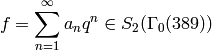
Example 9.15
The space
of cusp forms has dimension
and is spanned by two
-conjugate newforms, one of which is

where
. We will use Algorithm 9.14 to compute a few of these coefficients.
The space
of modular symbols has dimension
![[(0,0)],\quad [(1,0)], \quad [(0,1)],](_images/math/48962b2ac25543c14b6bf281bcb52ae49b90c69f.png)
where we use square brackets to differentiate Manin symbols from vectors. The Hecke operator
has characteristic polynomial
. The kernel of
corresponds to the span of the Eisenstein series of level
and weight
corresponds to
.) Each of the following steps corresponds to the step of Algorithm 9.14 with the same number.
- [Compute Projection] We compute projection onto
as in the algorithm). The matrix whose first two columns are the echelon basis for
and
so projection onto
[Choose
] Let  . Notice that
  ,
and
,
and ![v=[(1,0)]](_images/math/c41bb330b44348e764d9d463c387ae21a6e31654.png) is a sum of
only one Manin symbol.
is a sum of
only one Manin symbol.[Map from Hecke Ring] This step is purely conceptual, since no actual work needs to be done. We illustrate it by computing
 and
and  .
We have
.
We have
and

[Find Generator] We have
which is clearly independent from
 . Thus we
find that the image of the powers of
. Thus we
find that the image of the powers of  generate .
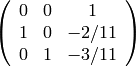
[Characteristic Polynomial] The matrix of
 is
is  , which has characteristic
polynomial
, which has characteristic
polynomial  . Of course, we already knew this because
we computed as the kernel of .
. Of course, we already knew this because
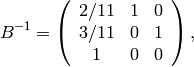
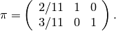
we computed as the kernel of .[Field Structure] We have

The matrix with rows the
 is
is  , which has inverse
  .
The matrix defines an isomorphism between and
the field
.
The matrix defines an isomorphism between and
the field![L=\Q[x]/(f) = \Q((-1+\sqrt{5})/2).](_images/math/31caf7df130f76e69deb412c736f0f0defbd63d6.png)
I.e.,
 and
and  , where
  .
.[Hecke Eigenvalues] We have
 . For example,
Example 9.16
It is easier to appreciate Algorithm 9.14 after seeing how big the coefficients of the power series expansion of a newform typically are, when the newform is defined over a large field. For example, there is a newform
such that if  , then
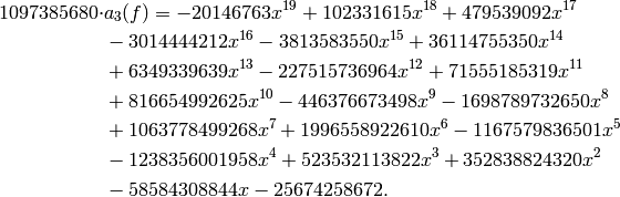
In contrast, if we take
 , then

Storing  as vectors
is more compact than storing
as vectors
is more compact than storing
 ,
,  ,
,  directly as polynomials in
  !
!
Congruences between Newforms
This section is about congruences between modular forms. Understanding congruences is crucial for studying Serre’s conjectures, Galois representations, and explicit construction of Hecke algebras. We assume more background in algebraic number theory here than elsewhere in this book.
Congruences between Modular Forms
Let  be an arbitrary congruence subgroup of
  ,
and suppose
,
and suppose  is a modular form of integer weight
for . Since
is a modular form of integer weight
for . Since  for some integer ,
the form has a Fourier expansion in
nonnegative powers of
for some integer ,
the form has a Fourier expansion in
nonnegative powers of  . For a rational
number , let
. For a rational
number , let  be the coefficient of
  in
the Fourier expansion of .
Put
in
the Fourier expansion of .
Put

where by convention we take  ,
so
,
so  .
.
The  -invariant
Let
be the -function,
which is a weight modular function
that is holomorphic except for a simple pole at  and
has integer Fourier coefficients (see, e.g.,
[Ser73, Section VIII.3.3]).
and
has integer Fourier coefficients (see, e.g.,
[Ser73, Section VIII.3.3]).
Lemma 9.17
Suppose  is a weight level
modular function that is holomorphic except possibly
with a pole of order at .
Then is a polynomial in of degree at most .
Moreover, the coefficients of this polynomial lie in
the ideal
is a weight level
modular function that is holomorphic except possibly
with a pole of order at .
Then is a polynomial in of degree at most .
Moreover, the coefficients of this polynomial lie in
the ideal  generated by the coefficients
  with
with  .
.
Proof
If  , then
  , so is constant with
constant term in , so the statement is true. Next suppose
, so is constant with
constant term in , so the statement is true. Next suppose  and the lemma
has been proved for all functions with smaller order poles.
Let
and the lemma
has been proved for all functions with smaller order poles.
Let  , and note that

Thus by induction  is a polynomial in
of degree
is a polynomial in
of degree  with coefficients in the ideal generated
by the coefficients with
with coefficients in the ideal generated
by the coefficients with  . It follows
that
. It follows
that  satisfies the conclusion
of the lemma.
satisfies the conclusion
of the lemma.
Sturm’s Theorem
If  is the ring of integers of a number field,
  is a maximal ideal of , and
 ![f=\sum a_n q^n \in \O[[q^{1/N}]]](_images/math/d1772c706fb58c32a5305cd2c53d2c38a3233c37.png) for some integer ,
let
for some integer ,
let

Note that  .
The following theorem was first proved in [Stu87].
.
The following theorem was first proved in [Stu87].
Theorem 9.18
Let be a prime ideal in the ring of integers of a
number field , and let be a congruence subgroup
of of index and level .
Suppose  is a modular form
and
is a modular form
and
or  is a cusp form
and
is a cusp form
and
Then  .
.
Proof
Case 1: First we assume  .
Let
.
Let

be the  function.
Since
function.
Since  , we have
  .
We have
.
We have
(4)
since is holomorphic at infinity and has a zero of order .
Also
(5)
Combining (4) and (5), we see that
with  and
and  if
if  .
.
By Lemma 9.17,
![f^{12} \cdot \Delta^{-k} \in \m[j]](_images/math/2c5cb9acf6cc96636663a56034caaf38b7141bd9.png)
is a polynomial in of degree at most with coefficients
in .
Thus
![f^{12} \in \m[j]\cdot \Delta^k,](_images/math/84ab08fa8031286209064bd97d91a23be0b2cbac.png)
so since the coefficients of are integers, every
coefficient of  is in . Thus
 hence
hence
 , so , as claimed.
Case 2: Arbitrary
Let be such that  , so also
 .
If
.
If  is arbitrary, then
because
is arbitrary, then
because  is a normal subgroup of ,
we have that for any
is a normal subgroup of ,
we have that for any  and
and  ,
,
![(g^{[\delta]_k})^{[\gamma]_k} = g^{[\delta\gamma]_k}
= g^{[\gamma'\delta]_k} = (g^{[\gamma']_k})^{[\delta]_k}
= g^{[\delta]_k},](_images/math/f9b53d468b58bcc2c4c7544b61d1ccb4187ff632.png)
where  . Thus for any
  ,
we have that
,
we have that ![g^{[\delta]_k} \in M_k(\Gamma(N))](_images/math/3111279588c55172d28fcea05a0e98212418ac8e.png) , so
acts on
, so
acts on  .
.
It is a standard (but nontrivial) fact about modular forms, which
comes from the geometry of the modular curve  over
over  and
and ![\Z[\zeta_N]](_images/math/fd2555c28a7d149d9eae9deaf661502d6df4ba52.png) , that has a basis with Fourier
expansions in
, that has a basis with Fourier
expansions in ![\Z[\zeta_N][[q^{1/N}]]](_images/math/d734ab779d2f2afb5fb5704cfc48d04980a86909.png) and that the action of
on preserves
and that the action of
on preserves
![M_k(\Gamma(N),\Q(\zeta_N)) = M_k(\Gamma(N)) \cap{}
(\Q(\zeta_N)[[q^{1/N}]])](_images/math/15021475c76cd150790d71bf6f0132258bfa06b8.png)
and the cuspidal subspace
 . In particular, for any
 ,
,
![f^{[\gamma]_k} \in M_k(\Gamma(N), K(\zeta_N))](_images/math/9c15b73652b634318028d3d4176c0a306485eca6.png)
Moreover, the denominators of ![f^{[\gamma]_k}](_images/math/6598c12197d74870e3b7b4f310ae83d100a42400.png) are bounded, since
is an
are bounded, since
is an ![\O[\zeta_N]](_images/math/8e97af206a4d40dbb5c23d7f69297cb99bf50b10.png) -linear combination of a basis for
-linear combination of a basis for
![M_k(\Gamma(N),\Z[\zeta_N])](_images/math/f08bbf8ef64d05850b33942f18614409e0201e71.png) , and the denominators of
divide the product of the denominators of the images of each of these
basis vectors under
, and the denominators of
divide the product of the denominators of the images of each of these
basis vectors under ![[\gamma]_k](_images/math/b982a736e025e060e88c63508ea36be04390f660.png) .
.
Let  .
Let
.
Let  be a prime of
  that divides
 . We will now show that for each , the
Chinese Remainder Theorem implies that there is an element
. We will now show that for each , the
Chinese Remainder Theorem implies that there is an element  such that
(6)![A_\gamma \cdot f^{[\gamma]_k} \in M_k(\Gamma(N), \O_L)
\qquad \text{and}
\qquad \ord_{\wM} (A_{\gamma} \cdot f^{[\gamma]_k}) < \infty.](_images/math/af0161390e80bf66285c5e8d02333071ec044bd0.png)
First find  such that
![A\cdot f^{[\gamma]_k}](_images/math/c06fb30ddfa5bcc9f4322119a1eb8a64ec720765.png) has coefficients in .
Choose
has coefficients in .
Choose  with
with  , and find a negative power
 such that
 ![\alpha^t\cdot A\cdot f^{[\gamma]_k}](_images/math/1e5d430a373980eff87f674bd3b68b5d6d8cc476.png) has -integral coefficients and finite valuation.
This is possible because we assumed that is nonzero.
Use the Chinese Remainder Theorem to find
has -integral coefficients and finite valuation.
This is possible because we assumed that is nonzero.
Use the Chinese Remainder Theorem to find  such that
  and
and  for each prime
  that divides
  .
Then for some
.
Then for some  we have
![\beta^s \cdot \alpha^t \cdot A\cdot f^{[\gamma]_k}
= A_\gamma \cdot f^{[\gamma]_k}
\in M_k(\Gamma(N),\O_L)](_images/math/fbd192d3c468f16ad4a892079388c9c19855e071.png)
and ![\ord_{\wM}(A_\gamma \cdot f^{[\gamma]_k}) < \infty](_images/math/89f0ef6badc3682b081f9970073ab3939cdfa99f.png) .
.
Write
with  , and let
![F = f \cdot \prod_{i=2}^m A_{\gamma_i} \cdot f^{[\gamma_i]_k}.](_images/math/29b456589a08c500642bac71dceb9575cd3c0c28.png)
Then  and since
  , we
have
, we
have 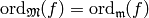 , so
, so
Thus we can apply Case 1 to conclude that
Thus
(7)![\infty = \ord_{\wM}(F) = \ord_\m(f) + \sum_{i=2}^m \ord_{\wM}(A_{\gamma_i}
f^{[\gamma]_k}),](_images/math/894af91a24f017c9b69930749dba139df238a632.png)
so  , because of (6).
We next obtain a better bound when is a cusp form.
Since preserves
cusp forms, ![\ord_{\wM}(A_{\gamma_i} f^{[\gamma]_k}) \geq \frac{1}{N}](_images/math/554fe22c959eca073331461601d8db4efecb1c49.png) for each
for each  .
Thus
.
Thus

since now we are merely assuming that

Thus we again apply Case 1 to conclude that
 and using (7), conclude that
.
and using (7), conclude that
.
Corollary 9.19
Let be a prime ideal in the ring of integers of a
number field. Suppose 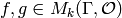 are modular
forms and
are modular
forms and

for all
where ![m=[\SL_2(\Z):\Gamma]](_images/math/ed667d3eecfa5190d947d52146b1212979c036d9.png) .
Then
.
Then 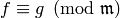 .
.
Buzzard proved the following corollary, which is extremely useful
in practical computations.
It asserts that the Sturm bound for modular forms with character
is the same as the Sturm bound for .
Corollary 9.20
Let be a prime ideal in the ring of integers of a
number field.
Suppose  are modular
forms with Dirichlet character
are modular
forms with Dirichlet character  and assume
that
and assume
that
where
![m=[\SL_2(\Z):\Gamma_0(N)] =
\#\P^1(\Z/N\Z) = N \cdot \prod_{p|N}\left(1+\frac{1}{p}\right).](_images/math/e49680865e13ec6570e88b88564f1dd786d8790f.png)
Then .
Proof
Let  and
let
and
let  ,
so
,
so  . Let be the order of the
Dirichlet character . Then
. Let be the order of the
Dirichlet character . Then  and
and
By Theorem 9.18, we have  ,
so
,
so  . It follows that .
Congruence for Newforms
Sturm’s paper [Stu87] also applies some results of Asai on
-expansions at various cusps to obtain a more refined result for
newforms.
Theorem 9.21
Let be a positive integer that is square-free, and
suppose and are two newforms in
 ,
where is the ring of integers of a number field,
and suppose that is a maximal ideal of .
Let be an arbitrary subset of the prime divisors of .
If
,
where is the ring of integers of a number field,
and suppose that is a maximal ideal of .
Let be an arbitrary subset of the prime divisors of .
If  for all
  and if

for all primes
![p \leq \frac{k\cdot [\SL_2(\Z):\Gamma_0(N)]}{12 \cdot 2^{\#I}},](_images/math/c12c977c2688bfe6507ea095381f96cc2342d3d9.png)
then .
The paper [BS02] contains a similar result about
congruences between newforms, which does not require that the level be
square-free. Recall from Definition Definition 4.18 that the
conductor of a Dirichlet character is the largest divisor  of such that factors through
  .
.
Theorem 9.22
Let  be any integer, and
suppose and are two normalized eigenforms in
be any integer, and
suppose and are two normalized eigenforms in  ,
where is the ring of integers of a number field,
and suppose that is a maximal ideal of .
Let be the set of prime divisors of that
do not divide
,
where is the ring of integers of a number field,
and suppose that is a maximal ideal of .
Let be the set of prime divisors of that
do not divide  .
If
.
If
for all primes and for all primes
then .
For the proof, see Lemma 1.4 and Corollary 1.7 in [BS02, Section 1.3].
Generating the Hecke Algebra
The following theorem appeared in [LS02, Appendix], except that
we give a better bound here. It is a nice application of the
congruence result above, which makes possible explicit computations
with Hecke rings .
Theorem 9.23
Suppose is a congruence subgroup that contains
and let
(8)
where .
Then the Hecke algebra
![\T=\Z[\ldots, T_n,\ldots] \subset \End(S_k(\Gamma))](_images/math/773b46e304024d8dbdf1477ce4fd6b1b5183d520.png)
is generated as a -module by the Hecke operators
for  .
.
Proof
For any ring  , let
, let  , where
![S_k(N;\Z)\subset \Z[[q]]](_images/math/51f1ec56f3a0cbbeb534a89ff9c4a351d5e14ae1.png) is the submodule of cusp forms with
integer Fourier expansion at the cusp , and let
is the submodule of cusp forms with
integer Fourier expansion at the cusp , and let  . For any ring , there is a perfect pairing
given by  (this is true
for
(this is true
for  , hence for any ).
Let be the submodule of  generated by
 , where
  is the largest integer
![\leq {\frac{kN}{12}}\cdot [\SL_2(\Z):\Gamma]](_images/math/52e72467050498603011d1e133dfa45ff21c58a4.png) .
Consider the exact sequence of additive abelian groups
.
Consider the exact sequence of additive abelian groups
Let be a prime and use the fact that
tensor product is right exact to obtain an exact sequence

Suppose that  pairs to with each of
 . Then

in  for each
  . By Theorem 9.18, it
follows that
. By Theorem 9.18, it
follows that  . Thus the pairing restricted to the image of
 in
in  is nondegenerate, so
because (8) is perfect, it follows that
is nondegenerate, so
because (8) is perfect, it follows that

Thus  .
Repeating the argument for all primes shows that
.
Repeating the argument for all primes shows that  ,
as claimed.
,
as claimed.
Remark 9.24
In general, the conclusion of
Theorem 9.23 is not true if one considers only
where runs over the primes less than the bound.
Consider, for example,  , where the bound is and
there are no primes
, where the bound is and
there are no primes  .
However, the Hecke algebra is generated as an algebra
by operators with
.
However, the Hecke algebra is generated as an algebra
by operators with  .
.
Exercises
Exercise 9.1
Prove that the group is a normal subgroup of
and that the quotient is
isomorphic to .
Exercise 9.2
Prove that the operators are elements of
![\Z[\ldots,T_n,\ldots]](_images/math/720b4867a6081836c716cd0c519d9c2148da5f20.png) . [Hint: Use Dirichlet’s theorem on primes in
arithmetic progression.]
. [Hint: Use Dirichlet’s theorem on primes in
arithmetic progression.]
Exercise 9.3
Find an example like Example 9.6 but in which the new subspace
is nonzero. More precisely, find an integer such that the Hecke
ring on  is not equal to the ring generated by
Hecke operators with and
is not equal to the ring generated by
Hecke operators with and
 .
.
Exercise 9.4
- Following Example 9.15, compute a basis for
 .
. - Use Algorithm 9.12 to compute a basis for
.
Footnotes
| [1] | John Cremona initially suggested to me the idea of separating these two maps. |